import rasterio
import numpy as np
import matplotlib.pyplot as plt
from rasterio.plot import show
print(f"Rasterio version: {rasterio.__version__}")
Rasterio version: 1.4.3Rasterio is the essential Python library for reading and writing geospatial raster data.
import rasterio
import numpy as np
import matplotlib.pyplot as plt
from rasterio.plot import show
print(f"Rasterio version: {rasterio.__version__}")Rasterio version: 1.4.3Since we may not have actual satellite imagery files, let’s create some sample raster data:
# Create sample raster data
def create_sample_raster():
    # Create a simple 100x100 raster with some pattern
    height, width = 100, 100

    # Create coordinate grids
    x = np.linspace(-2, 2, width)
    y = np.linspace(-2, 2, height)
    X, Y = np.meshgrid(x, y)

    # Create a pattern (e.g., circular pattern)
    data = np.sin(np.sqrt(X**2 + Y**2)) * 255
    data = data.astype(np.uint8)

    return data

sample_data = create_sample_raster()
print(f"Sample data shape: {sample_data.shape}")
print(f"Data type: {sample_data.dtype}")
print(f"Data range: {sample_data.min()} to {sample_data.max()}")
Sample data shape: (100, 100)
Data type: uint8
Data range: 7 to 254# Basic statistics
print(f"Mean: {np.mean(sample_data):.2f}")
print(f"Standard deviation: {np.std(sample_data):.2f}")
print(f"Unique values: {len(np.unique(sample_data))}")
# Histogram of values
plt.figure(figsize=(8, 4))
plt.subplot(1, 2, 1)
plt.imshow(sample_data, cmap='viridis')
plt.title('Sample Raster Data')
plt.colorbar()
plt.subplot(1, 2, 2)
plt.hist(sample_data.flatten(), bins=50, alpha=0.7)
plt.title('Histogram of Values')
plt.xlabel('Pixel Value')
plt.ylabel('Frequency')
plt.tight_layout()
plt.show()Mean: 215.01
Standard deviation: 46.13
Unique values: 182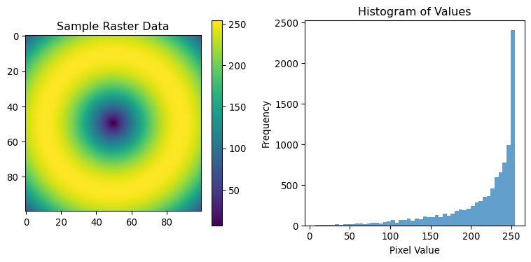
# Create masks
high_values = sample_data > 200
low_values = sample_data < 50

print(f"Pixels with high values (>200): {np.sum(high_values)}")
print(f"Pixels with low values (<50): {np.sum(low_values)}")

# Apply mask
masked_data = np.where(high_values, sample_data, 0)

plt.figure(figsize=(12, 4))

plt.subplot(1, 3, 1)
plt.imshow(sample_data, cmap='viridis')
plt.title('Original Data')

plt.subplot(1, 3, 2)
plt.imshow(high_values, cmap='gray')
plt.title('High Value Mask')

plt.subplot(1, 3, 3)
plt.imshow(masked_data, cmap='viridis')
plt.title('Masked Data')

plt.tight_layout()
plt.show()
Pixels with high values (>200): 7364
Pixels with low values (<50): 76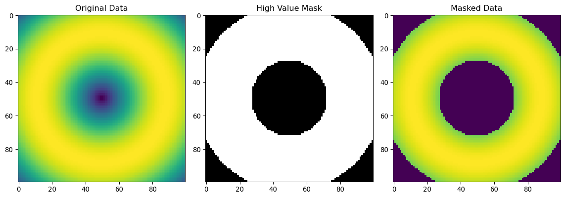
from rasterio.transform import from_bounds

# Create a sample transform (geographic coordinates)
west, south, east, north = -120.0, 35.0, -115.0, 40.0  # Bounding box
transform = from_bounds(west, south, east, north, 100, 100)

print(f"Transform: {transform}")
print(f"Pixel width: {transform[0]}")
print(f"Pixel height: {abs(transform[4])}")

# Convert pixel coordinates to geographic coordinates
def pixel_to_geo(row, col, transform):
    x, y = rasterio.transform.xy(transform, row, col)
    return x, y

# Example: center pixel
center_row, center_col = 50, 50
geo_x, geo_y = pixel_to_geo(center_row, center_col, transform)
print(f"Center pixel ({center_row}, {center_col}) -> Geographic: ({geo_x:.2f}, {geo_y:.2f})")
Transform: | 0.05, 0.00,-120.00|
| 0.00,-0.05, 40.00|
| 0.00, 0.00, 1.00|
Pixel width: 0.05
Pixel height: 0.05
Center pixel (50, 50) -> Geographic: (-117.47, 37.48)# Create a profile for writing raster data
profile = {
'driver': 'GTiff',
'dtype': 'uint8',
'nodata': None,
'width': 100,
'height': 100,
'count': 1,
'crs': 'EPSG:4326', # WGS84 lat/lon
'transform': transform
}
print("Raster profile:")
for key, value in profile.items():
print(f" {key}: {value}")Raster profile:
driver: GTiff
dtype: uint8
nodata: None
width: 100
height: 100
count: 1
crs: EPSG:4326
transform: | 0.05, 0.00,-120.00|
| 0.00,-0.05, 40.00|
| 0.00, 0.00, 1.00|# Create multi-band sample data (RGB-like)
def create_multiband_sample():
height, width = 100, 100
bands = 3
# Create different patterns for each band
x = np.linspace(-2, 2, width)
y = np.linspace(-2, 2, height)
X, Y = np.meshgrid(x, y)
# Band 1: Circular pattern
band1 = (np.sin(np.sqrt(X**2 + Y**2)) * 127 + 127).astype(np.uint8)
# Band 2: Linear gradient
band2 = (np.linspace(0, 255, width) * np.ones((height, 1))).astype(np.uint8)
# Band 3: Checkerboard pattern
band3 = ((X + Y) > 0).astype(np.uint8) * 255
return np.stack([band1, band2, band3])
multiband_data = create_multiband_sample()
print(f"Multiband shape: {multiband_data.shape}")
print(f"Shape format: (bands, height, width)")Multiband shape: (3, 100, 100)
Shape format: (bands, height, width)fig, axes = plt.subplots(2, 2, figsize=(10, 10))
# Individual bands
for i in range(3):
row, col = i // 2, i % 2
axes[row, col].imshow(multiband_data[i], cmap='gray')
axes[row, col].set_title(f'Band {i+1}')
# RGB composite (transpose for matplotlib)
rgb_composite = np.transpose(multiband_data, (1, 2, 0))
axes[1, 1].imshow(rgb_composite)
axes[1, 1].set_title('RGB Composite')
plt.tight_layout()
plt.show()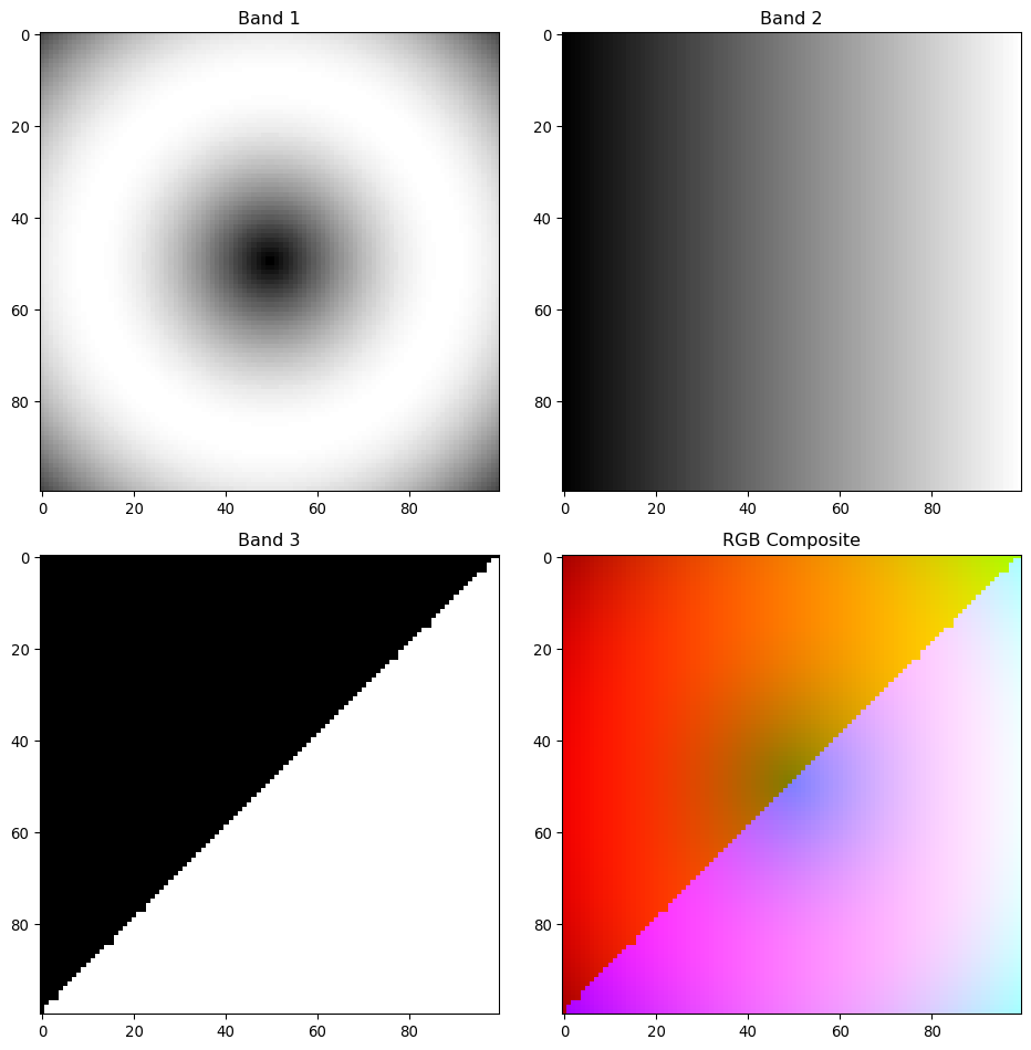
# Simulate NIR and Red bands
nir_band = multiband_data[0].astype(np.float32)
red_band = multiband_data[1].astype(np.float32)

# Calculate NDVI-like index
# NDVI = (NIR - Red) / (NIR + Red)
ndvi = (nir_band - red_band) / (nir_band + red_band + 1e-8)  # Small value to avoid division by zero

plt.figure(figsize=(12, 4))

plt.subplot(1, 3, 1)
plt.imshow(nir_band, cmap='RdYlBu_r')
plt.title('NIR-like Band')
plt.colorbar()

plt.subplot(1, 3, 2)
plt.imshow(red_band, cmap='Reds')
plt.title('Red-like Band')
plt.colorbar()

plt.subplot(1, 3, 3)
plt.imshow(ndvi, cmap='RdYlGn', vmin=-1, vmax=1)
plt.title('NDVI-like Index')
plt.colorbar()

plt.tight_layout()
plt.show()

print(f"NDVI range: {ndvi.min():.3f} to {ndvi.max():.3f}")
print(f"NDVI mean: {np.mean(ndvi):.3f}")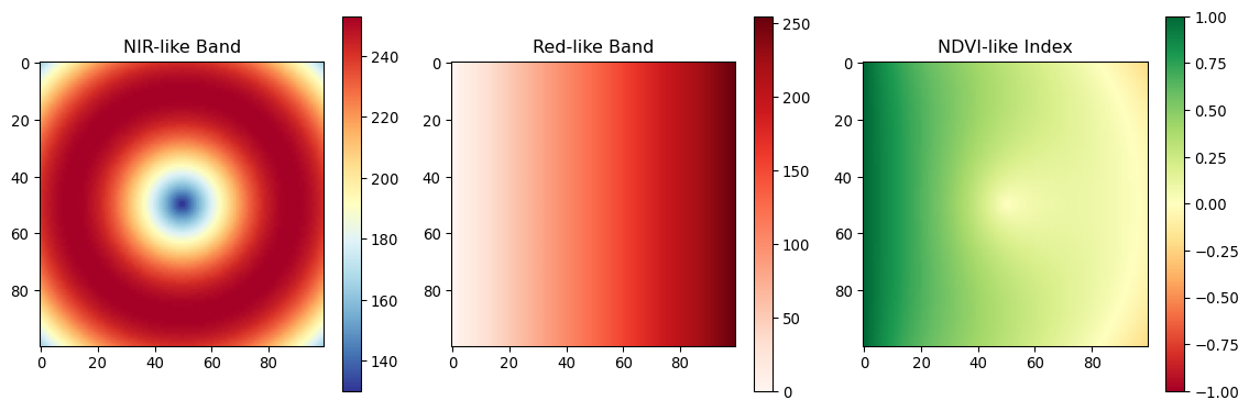
NDVI range: -0.211 to 1.000
NDVI mean: 0.353from scipy import ndimage
# Demonstrate different resampling methods
original = sample_data
# Downsample (reduce resolution)
downsampled = ndimage.zoom(original, 0.5, order=1) # Linear interpolation
# Upsample (increase resolution)
upsampled = ndimage.zoom(original, 2.0, order=1) # Linear interpolation
plt.figure(figsize=(15, 4))
plt.subplot(1, 3, 1)
plt.imshow(original, cmap='viridis')
plt.title(f'Original ({original.shape[0]}x{original.shape[1]})')
plt.subplot(1, 3, 2)
plt.imshow(downsampled, cmap='viridis')
plt.title(f'Downsampled ({downsampled.shape[0]}x{downsampled.shape[1]})')
plt.subplot(1, 3, 3)
plt.imshow(upsampled, cmap='viridis')
plt.title(f'Upsampled ({upsampled.shape[0]}x{upsampled.shape[1]})')
plt.tight_layout()
plt.show()
print(f"Original size: {original.shape}")
print(f"Downsampled size: {downsampled.shape}")
print(f"Upsampled size: {upsampled.shape}")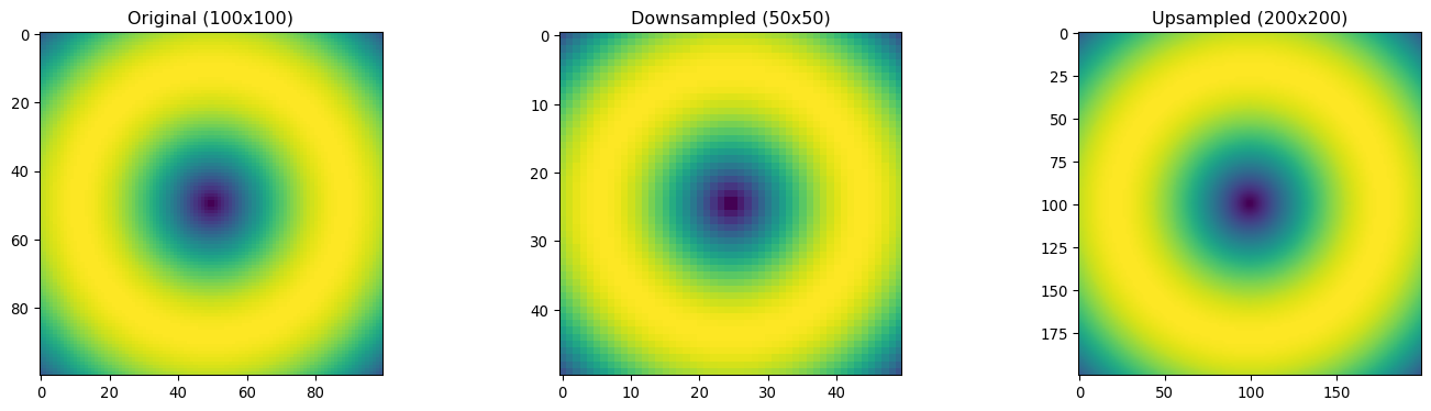
Original size: (100, 100)
Downsampled size: (50, 50)
Upsampled size: (200, 200)# Simulate processing large rasters in blocks
def process_in_blocks(data, block_size=50):
"""Process data in blocks to simulate handling large rasters"""
height, width = data.shape
processed = np.zeros_like(data)
for row in range(0, height, block_size):
for col in range(0, width, block_size):
# Define window bounds
row_end = min(row + block_size, height)
col_end = min(col + block_size, width)
# Extract block
block = data[row:row_end, col:col_end]
# Process block (example: enhance contrast)
processed_block = np.clip(block * 1.2, 0, 255)
# Write back to result
processed[row:row_end, col:col_end] = processed_block
print(f"Processed block: ({row}:{row_end}, {col}:{col_end})")
return processed
# Process sample data in blocks
processed_data = process_in_blocks(sample_data, block_size=25)
plt.figure(figsize=(10, 4))
plt.subplot(1, 2, 1)
plt.imshow(sample_data, cmap='viridis')
plt.title('Original')
plt.subplot(1, 2, 2)
plt.imshow(processed_data, cmap='viridis')
plt.title('Processed (Enhanced)')
plt.tight_layout()
plt.show()Processed block: (0:25, 0:25)
Processed block: (0:25, 25:50)
Processed block: (0:25, 50:75)
Processed block: (0:25, 75:100)
Processed block: (25:50, 0:25)
Processed block: (25:50, 25:50)
Processed block: (25:50, 50:75)
Processed block: (25:50, 75:100)
Processed block: (50:75, 0:25)
Processed block: (50:75, 25:50)
Processed block: (50:75, 50:75)
Processed block: (50:75, 75:100)
Processed block: (75:100, 0:25)
Processed block: (75:100, 25:50)
Processed block: (75:100, 50:75)
Processed block: (75:100, 75:100)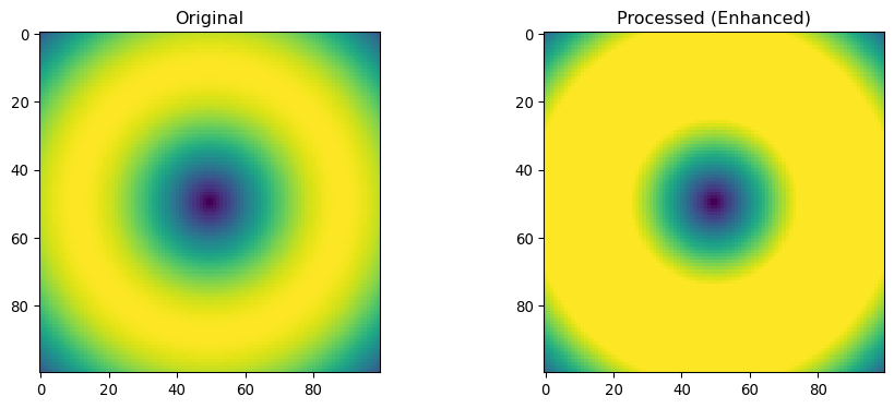
Key Rasterio concepts covered: - Reading and understanding raster data structure - Working with single and multi-band imagery - Coordinate transforms and geospatial metadata
- Band math and index calculations - Resampling and processing techniques - Block-based processing for large datasets