Foundation models represent a paradigm shift in machine learning, where large-scale models are trained on diverse, unlabeled data and then adapted to various downstream tasks. The term was coined by the Stanford HAI Center to describe models like GPT-3, BERT, and CLIP that serve as a “foundation” for numerous applications.
This cheatsheet provides a comprehensive comparison between Language Models (LLMs) and Geospatial Foundation Models (GFMs), examining their architectures, training procedures, and deployment strategies. While LLMs process discrete text tokens, GFMs work with continuous multi-spectral imagery, requiring fundamentally different approaches to tokenization, positional encoding, and objective functions.
PyTorch version: 2.7.1
CUDA available: False
MPS available: True
Using device: mps
Evolution from AI to Transformers
The development of foundation models represents a convergence of several key technological breakthroughs. The journey from symbolic AI to modern foundation models reflects both advances in computational power and fundamental insights about learning representations from large-scale data.
Key Historical Milestones
The transformer architecture emerged from decades of research in neural networks, attention mechanisms, and sequence modeling. The 2017 paper “Attention Is All You Need” introduced the transformer, which became the foundation for both language and vision models.
Critical Developments:
1950s-1990s: Symbolic AI dominated, with rule-based systems and early neural networks
2017: The Transformer architecture introduced self-attention and parallelizable training
2018-2020: BERT and GPT families demonstrated the power of pre-trained language models
2021-2024: Scaling laws, ChatGPT, and multimodal models like CLIP
Foundation Model Evolution Timeline:
2017 - Transformer: Base architecture introduced
2018 - BERT-Base: 110M parameters
2019 - GPT-2: 1.5B parameters
2020 - GPT-3: 175B parameters
2021 - ViT-Large: 307M parameters for vision
2022 - PaLM: 540B parameters
2023 - GPT-4: ~1T parameters (estimated)
2024 - Claude-3: Multi-modal capabilities
Transformer Architecture Essentials
The transformer architecture revolutionized deep learning by introducing the self-attention mechanism, which allows models to process sequences in parallel rather than sequentially. This architecture forms the backbone of both language models (GPT, BERT) and vision models (ViT, DINO).
Core Components:
Multi-Head Attention: Allows the model to attend to different representation subspaces (see Self-attention)
Feed-Forward Networks: Point-wise processing with GELU activation (see Multilayer perceptron)
Layer Normalization: Stabilizes training and improves convergence (see Layer normalization)
Key terms (quick definitions):
Self-Attention (SA): A mechanism where each token attends to every other token (including itself) to compute a weighted combination of their representations.
Queries (Q), Keys (K), Values (V): Learned linear projections of the input. Attention scores are computed from Q·Kᵀ; those scores weight V to produce the output (see Attention (machine learning)).
Multi-Head Attention (MHA): Runs several SA “heads” in parallel on different subspaces, then concatenates and projects the results. This lets the model capture diverse relationships (see Self-attention).
Feed-Forward Network (FFN/MLP): A small two-layer MLP (Multi-Layer Perceptron) applied to each token independently; expands the dimension then projects back (often with GELU activation) (see Multilayer perceptron).
Residual Connection (Skip): Adds the input of a sub-layer to its output, helping gradients flow and preserving information (see Residual neural network).
Layer Normalization (LayerNorm, LN): Normalizes features per token to stabilize training. The ordering with residuals defines Post-LN vs Pre-LN variants (see Layer normalization).
GELU: Gaussian Error Linear Unit activation; smoother than ReLU and standard in transformers (see Gaussian error linear unit).
Tensor shape convention: Using batch_first=True, tensors are [batch_size, seq_len, embed_dim].
Abbreviations used: B = batch size, S = sequence length (or number of tokens/patches), E = embedding dimension, H = number of attention heads.
The following implementation demonstrates a simplified transformer block following the original architecture:
class SimpleTransformerBlock(nn.Module):"""Transformer block with Multi-Head Self-Attention (MHSA) and MLP. Inputs/Outputs: - x: [batch_size, seq_len, embed_dim] - returns: same shape as input Structure (Post-LN variant): x = LN(x + MHSA(x)) x = LN(x + MLP(x)) """def__init__(self, embed_dim=768, num_heads=8, mlp_ratio=4):super().__init__()self.embed_dim = embed_dim# Multi-Head Self-Attention (MHSA)# - batch_first=True → tensors are [B, S, E]# - Self-attention uses Q=K=V=linear(x) by defaultself.attention = nn.MultiheadAttention( embed_dim=embed_dim, num_heads=num_heads, batch_first=True, )# Position-wise feed-forward network (applied independently to each token) hidden_dim =int(embed_dim * mlp_ratio)self.mlp = nn.Sequential( nn.Linear(embed_dim, hidden_dim), # expand nn.GELU(), # nonlinearity nn.Linear(hidden_dim, embed_dim), # project back )# LayerNorms used after residual additions (Post-LN)self.norm1 = nn.LayerNorm(embed_dim)self.norm2 = nn.LayerNorm(embed_dim)def forward(self, x: torch.Tensor) -> torch.Tensor:# x: [B, S, E]# Multi-head self-attention# attn_out: [B, S, E]; attn_weights (ignored here) would be [B, num_heads, S, S] attn_out, _ =self.attention(x, x, x) # Q=K=V=x (self-attention)# Residual connection + LayerNorm (Post-LN) x =self.norm1(x + attn_out)# Position-wise MLP mlp_out =self.mlp(x) # [B, S, E]# Residual connection + LayerNorm (Post-LN) x =self.norm2(x + mlp_out)return x # shape preserved: [B, S, E]# Example usage and shape checkstransformer_block = SimpleTransformerBlock(embed_dim=768, num_heads=8)sample_input = torch.randn(2, 100, 768) # [batch_size, seq_len, embed_dim]output = transformer_block(sample_input)print(f"Input shape: {sample_input.shape}")print(f"Output shape: {output.shape}") # should match inputprint(f"Parameters: {sum(p.numel() for p in transformer_block.parameters()):,}")
What to notice: - Shapes are stable through the block: [B, S, E] → [B, S, E]. - Residuals + LayerNorm appear after each sublayer (Post-LN variant). - MLP expands to mlp_ratio × embed_dim then projects back.
LLMs vs GFMs
Both LLMs and GFMs follow similar high-level development pipelines, but differ in the details because language and satellite imagery are very different kinds of data.
9-Step Development Pipeline Comparison
Data Preparation: Gather raw data and clean it up so the model can learn useful patterns.
Tokenization (turning inputs into pieces the model can handle): Decide how to chop inputs into small parts the model can process.
Architecture (the model blueprint): Choose how many layers, how wide/tall the model is, and how it connects information.
Pretraining Objective (what the model practices): Pick the learning task the model does before any specific application.
Training Loop (how learning happens): Decide optimizers, learning rate, precision, and how to stabilize training.
Evaluation (how we check learning): Use simple tests to see if the model is improving in the right ways.
Pretrained Weights (starting point): Load existing model parameters to avoid training from scratch.
Finetuning (adapting the model): Add a small head or nudge the model for a specific task with labeled examples.
Deployment (using the model in practice): Serve the model efficiently and handle real-world input sizes.
LLM Development Pipeline
Language models like GPT and BERT have established a mature development pipeline refined through years of research. The process emphasizes text quality, vocabulary optimization, and language understanding benchmarks.
Geospatial foundation models adapt the transformer architecture for Earth observation data, requiring specialized handling of multi-spectral imagery, temporal sequences, and spatial relationships.
Collect large text sets, remove duplicates and low-quality content
Collect scenes from sensors, correct for atmosphere/sensor, remove clouds, tile into manageable chips
2. Tokenization
Break text into subword tokens; build a vocabulary
Cut images into patches; turn each patch into a vector; add 2D (and time) positions
3. Architecture
Transformer layers over token sequences (often decoder-only for GPT, encoder-only for BERT)
Vision Transformer-style encoders over patch sequences; may include temporal attention for time series
4. Pretraining Objective
Predict the next/missing word to learn language patterns
Reconstruct masked image patches or learn similarities across views/time to learn visual patterns
5. Training Loop
AdamW, learning-rate schedule, mixed precision; long sequences can stress memory
Similar tools, but memory shaped by patch size, bands, and image tiling; may mask clouds or invalid pixels
6. Evaluation
Quick checks like “how surprised is the model?” (e.g., next-word loss) and small downstream tasks
Quick checks like reconstruction quality and small downstream tasks (e.g., linear probes on land cover)
7. Pretrained Weights
Download weights and matching tokenizer from model hubs
Download weights from hubs (e.g., Prithvi, SatMAE); ensure band order and preprocessing match
8. Finetuning
Add a small head or adapters; few labeled examples can go far
Add a task head (classification/segmentation); often freeze encoder and train a light head on small datasets
9. Deployment
Serve via APIs; speed up with caching of past context
Run sliding-window/tiling over large scenes; export results as geospatial rasters/vectors
Step-by-Step Detailed Comparison
Let’s look at more detailed comparisons beetween each development pipeline step, highlighting the fundamental differences between text and geospatial data processing.
Data Preparation Differences
Data preparation represents one of the most significant differences between LLMs and GFMs. LLMs work with human-generated text that requires quality filtering and deduplication, while GFMs process sensor data that requires physical corrections and calibration.
LLM Data Challenges:
Scale: Training datasets like CommonCrawl contain hundreds of terabytes
Quality: Filtering toxic content, spam, and low-quality text
Deduplication: Removing exact and near-duplicate documents
Language Detection: Identifying and filtering by language
GFM Data Challenges:
Sensor Calibration: Converting raw digital numbers to physical units
Atmospheric Correction: Removing atmospheric effects from satellite imagery
Cloud Masking: Identifying and handling cloudy pixels
Georegistration: Aligning images to geographic coordinate systems
# LLM text preprocessing examplesample_texts = ["The quick brown fox jumps over the lazy dog.","Machine learning is transforming many industries.", "Climate change requires urgent global action."]# Basic tokenization for vocabulary constructionvocab =set()for text in sample_texts: vocab.update(text.lower().replace('.', '').split())print("LLM Data Processing:")print(f"Sample vocabulary size: {len(vocab)}")print(f"Sample tokens: {list(vocab)[:10]}")print("\n"+"="*50+"\n")# GFM satellite data preprocessing examplenp.random.seed(42)patch_size =64num_bands =6# Simulate raw satellite patch (typical 12-bit values)satellite_patch = np.random.randint(0, 4096, (num_bands, patch_size, patch_size))# Simulate cloud mask (20% cloud coverage)cloud_mask = np.random.random((patch_size, patch_size)) >0.8# Apply atmospheric correction (normalize to [0,1])corrected_patch = satellite_patch.astype(np.float32) /4095.0corrected_patch[:, cloud_mask] = np.nan # Mask cloudy pixelsprint("GFM Data Processing:")print(f"Satellite patch shape: {satellite_patch.shape} (bands, height, width)")print(f"Cloud coverage: {cloud_mask.sum() / cloud_mask.size *100:.1f}%")print(f"Valid pixels per band: {(~np.isnan(corrected_patch[0])).sum():,}")
Tokenization represents a fundamental difference between language and vision models. LLMs use discrete tokenization with learned vocabularies (like BPE), while GFMs use continuous tokenization through patch embeddings inspired by Vision Transformers.
LLM Tokenization:
Byte-Pair Encoding (BPE): Learns subword units to handle out-of-vocabulary words
Vocabulary Size: Typically 30K-100K tokens balancing efficiency and coverage
Special Tokens: [CLS], [SEP], [PAD], [MASK] for different tasks
GFM Tokenization:
Patch Embedding: Divides images into fixed-size patches (e.g., 16×16 pixels)
Linear Projection: Maps high-dimensional patches to embedding space
Positional Encoding: 2D spatial positions rather than 1D sequence positions
While both LLMs and GFMs use transformer architectures, they differ in input processing, positional encoding, and output heads. LLMs like GPT use causal attention for autoregressive generation, while GFMs like Prithvi use bidirectional attention for representation learning.
Key Architectural Differences:
Input Processing: 1D token sequences vs. 2D spatial patches
Positional Encoding: 1D learned positions vs. 2D spatial coordinates
Attention Patterns: Causal masking vs. full bidirectional attention
Output Heads: Language modeling head vs. reconstruction/classification heads
The pretraining objectives differ fundamentally between text and visual domains. LLMs excel at predictive modeling (predicting the next token), while GFMs focus on reconstructive modeling (rebuilding masked image patches).
LLM Objectives:
Next-Token Prediction: GPT-style autoregressive modeling for text generation
Masked Language Modeling: BERT-style bidirectional understanding
Instruction Following: Learning to follow human instructions (InstructGPT)
GFM Objectives:
Masked Patch Reconstruction: MAE-style learning of visual representations
Contrastive Learning: Learning invariances across time and space (SimCLR, CLIP)
Multi-task Pretraining: Combining reconstruction with auxiliary tasks
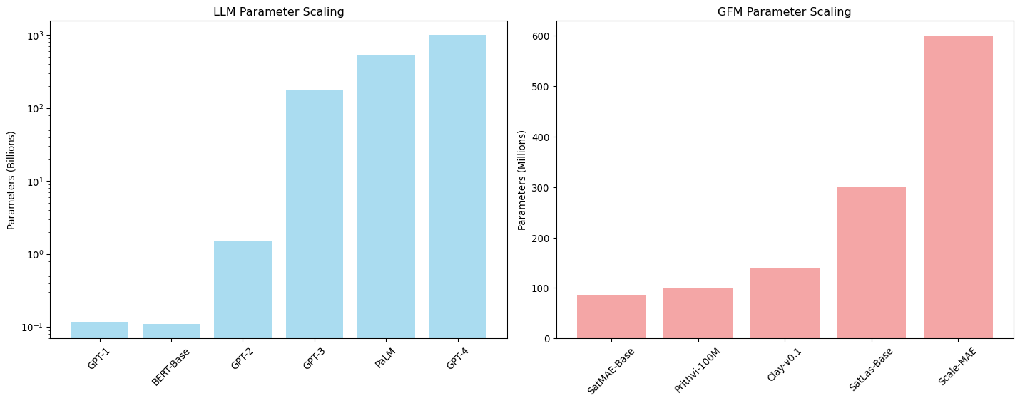
The scaling trends between LLMs and GFMs reveal different optimization strategies. LLMs focus on parameter scaling (billions of parameters) while GFMs emphasize data modality scaling (spectral, spatial, and temporal dimensions).
The data infrastructure requirements for LLMs and GFMs differ dramatically due to the nature of text versus imagery data. Understanding these constraints is crucial for development planning.
Aspect
LLMs
GFMs
Data Volume
Terabytes of text data (web crawls, books, code repositories)
Petabytes of satellite imagery (constrained by storage/IO bandwidth)
Data Quality Challenges
Deduplication algorithms, toxicity filtering, language detection
Embeddings are the foundation of both LLMs and GFMs, but they differ in how raw inputs are converted to dense vector representations. This section demonstrates practical implementation patterns for both domains.
# Text embedding creation (LLM approach)text ="The forest shows signs of deforestation."tokens = text.lower().replace('.', '').split()# Create simple vocabulary mappingvocab = {word: i for i, word inenumerate(set(tokens))}vocab['<PAD>'] =len(vocab)vocab['<UNK>'] =len(vocab)# Convert text to token IDstoken_ids = [vocab.get(token, vocab['<UNK>']) for token in tokens]token_tensor = torch.tensor(token_ids).unsqueeze(0)# Embedding layer lookupembed_layer = nn.Embedding(len(vocab), 256)text_embeddings = embed_layer(token_tensor)print("Text Embeddings (LLM):")print(f"Original text: {text}")print(f"Tokens: {tokens}")print(f"Token IDs: {token_ids}")print(f"Embeddings shape: {text_embeddings.shape}")print("\n"+"-"*50+"\n")# Patch embedding creation (GFM approach)patch_size =16num_bands =6# Create sample multi-spectral satellite patchsatellite_patch = torch.randn(1, num_bands, patch_size, patch_size)# Flatten patch for linear projectionpatch_flat = satellite_patch.view(1, num_bands * patch_size * patch_size)# Linear projection to embedding spacepatch_projection = nn.Linear(num_bands * patch_size * patch_size, 256)patch_embeddings = patch_projection(patch_flat)print("Patch Embeddings (GFM):")print(f"Original patch shape: {satellite_patch.shape}")print(f"Flattened patch shape: {patch_flat.shape}")print(f"Patch embeddings shape: {patch_embeddings.shape}")
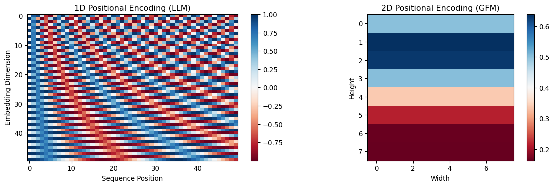
Positional encodings enable transformers to understand sequence order (LLMs) or spatial relationships (GFMs). The fundamental difference lies in 1D sequential positions versus 2D spatial coordinates.
Key Differences:
LLM: 1D sinusoidal encoding for sequence positions
---title: "Foundation Model Architectures"subtitle: "LLMs vs. Geospatial Foundation Models (GFMs)"jupyter: geoaiformat: html: toc: true toc-depth: 3---## Introduction to Foundation Model ArchitecturesFoundation models represent a paradigm shift in machine learning, where large-scale models are trained on diverse, unlabeled data and then adapted to various downstream tasks. The term was coined by the [Stanford HAI Center](https://hai.stanford.edu/news/reflections-foundation-models) to describe models like GPT-3, BERT, and CLIP that serve as a "foundation" for numerous applications.This cheatsheet provides a comprehensive comparison between **Language Models (LLMs)** and **Geospatial Foundation Models (GFMs)**, examining their architectures, training procedures, and deployment strategies. While LLMs process discrete text tokens, GFMs work with continuous multi-spectral imagery, requiring fundamentally different approaches to tokenization, positional encoding, and objective functions.**Key Resources:**- [Attention Is All You Need](https://arxiv.org/abs/1706.03762) - Original Transformer paper- [An Image is Worth 16x16 Words](https://arxiv.org/abs/2010.11929) - Vision Transformer (ViT)- [Masked Autoencoders Are Scalable Vision Learners](https://arxiv.org/abs/2111.06377) - MAE approach- [Prithvi Foundation Model](https://huggingface.co/ibm-nasa-geospatial/Prithvi-100M) - IBM/NASA geospatial model### Setup```{python}import torchimport torch.nn as nnimport numpy as npimport matplotlib.pyplot as pltfrom transformers import AutoModel, AutoConfigprint(f"PyTorch version: {torch.__version__}")print(f"CUDA available: {torch.cuda.is_available()}") # Always False on Macmps_available = torch.backends.mps.is_available()print(f"MPS available: {mps_available}")if mps_available: device = torch.device("mps")elif torch.cuda.is_available(): device = torch.device("cuda")else: device = torch.device("cpu")print(f"Using device: {device}")```### Evolution from AI to TransformersThe development of foundation models represents a convergence of several key technological breakthroughs. The journey from symbolic AI to modern foundation models reflects both advances in computational power and fundamental insights about learning representations from large-scale data.#### Key Historical MilestonesThe transformer architecture emerged from decades of research in neural networks, attention mechanisms, and sequence modeling. The 2017 paper "[Attention Is All You Need](https://arxiv.org/abs/1706.03762)" introduced the transformer, which became the foundation for both language and vision models.**Critical Developments:**- **1950s-1990s**: Symbolic AI dominated, with rule-based systems and early neural networks- **2012**: [AlexNet's ImageNet victory](https://papers.nips.cc/paper/2012/hash/c399862d3b9d6b76c8436e924a68c45b-Abstract.html) sparked the deep learning revolution- **2017**: The Transformer architecture introduced self-attention and parallelizable training- **2018-2020**: BERT and GPT families demonstrated the power of pre-trained language models- **2021-2024**: Scaling laws, [ChatGPT](https://openai.com/blog/chatgpt), and multimodal models like [CLIP](https://arxiv.org/abs/2103.00020)**Foundation Model Evolution Timeline:**- **2017 - Transformer**: Base architecture introduced- **2018 - BERT-Base**: 110M parameters- **2019 - GPT-2**: 1.5B parameters - **2020 - GPT-3**: 175B parameters- **2021 - ViT-Large**: 307M parameters for vision- **2022 - PaLM**: 540B parameters- **2023 - GPT-4**: ~1T parameters (estimated)- **2024 - Claude-3**: Multi-modal capabilities### Transformer Architecture EssentialsThe transformer architecture revolutionized deep learning by introducing the **self-attention mechanism**, which allows models to process sequences in parallel rather than sequentially. This architecture forms the backbone of both language models (GPT, BERT) and vision models (ViT, DINO).**Core Components:**- **Multi-Head Attention**: Allows the model to attend to different representation subspaces (see [Self-attention](https://en.wikipedia.org/wiki/Self-attention))- **Feed-Forward Networks**: Point-wise processing with GELU activation (see [Multilayer perceptron](https://en.wikipedia.org/wiki/Multilayer_perceptron))- **Residual Connections**: Enable training of very deep networks (see [Residual neural network](https://en.wikipedia.org/wiki/Residual_neural_network))- **Layer Normalization**: Stabilizes training and improves convergence (see [Layer normalization](https://en.wikipedia.org/wiki/Layer_normalization))**Key terms (quick definitions):**- **Self-Attention (SA)**: A mechanism where each token attends to every other token (including itself) to compute a weighted combination of their representations.- **Queries (Q), Keys (K), Values (V)**: Learned linear projections of the input. Attention scores are computed from Q·Kᵀ; those scores weight V to produce the output (see [Attention (machine learning)](https://en.wikipedia.org/wiki/Attention_(machine_learning))).- **Multi-Head Attention (MHA)**: Runs several SA “heads” in parallel on different subspaces, then concatenates and projects the results. This lets the model capture diverse relationships (see [Self-attention](https://en.wikipedia.org/wiki/Self-attention)).- **Feed-Forward Network (FFN/MLP)**: A small two-layer MLP (Multi-Layer Perceptron) applied to each token independently; expands the dimension then projects back (often with GELU activation) (see [Multilayer perceptron](https://en.wikipedia.org/wiki/Multilayer_perceptron)).- **Residual Connection (Skip)**: Adds the input of a sub-layer to its output, helping gradients flow and preserving information (see [Residual neural network](https://en.wikipedia.org/wiki/Residual_neural_network)).- **Layer Normalization (LayerNorm, LN)**: Normalizes features per token to stabilize training. The ordering with residuals defines Post-LN vs Pre-LN variants (see [Layer normalization](https://en.wikipedia.org/wiki/Layer_normalization)).- **GELU**: Gaussian Error Linear Unit activation; smoother than ReLU and standard in transformers (see [Gaussian error linear unit](https://en.wikipedia.org/wiki/Activation_function#Gaussian_error_linear_unit_(GELU))).- **Tensor shape convention**: Using `batch_first=True`, tensors are `[batch_size, seq_len, embed_dim]`.- **Abbreviations used**: `B` = batch size, `S` = sequence length (or number of tokens/patches), `E` = embedding dimension, `H` = number of attention heads.The following implementation demonstrates a simplified transformer block following the [original architecture](https://arxiv.org/abs/1706.03762):```{python}class SimpleTransformerBlock(nn.Module):"""Transformer block with Multi-Head Self-Attention (MHSA) and MLP. Inputs/Outputs: - x: [batch_size, seq_len, embed_dim] - returns: same shape as input Structure (Post-LN variant): x = LN(x + MHSA(x)) x = LN(x + MLP(x)) """def__init__(self, embed_dim=768, num_heads=8, mlp_ratio=4):super().__init__()self.embed_dim = embed_dim# Multi-Head Self-Attention (MHSA)# - batch_first=True → tensors are [B, S, E]# - Self-attention uses Q=K=V=linear(x) by defaultself.attention = nn.MultiheadAttention( embed_dim=embed_dim, num_heads=num_heads, batch_first=True, )# Position-wise feed-forward network (applied independently to each token) hidden_dim =int(embed_dim * mlp_ratio)self.mlp = nn.Sequential( nn.Linear(embed_dim, hidden_dim), # expand nn.GELU(), # nonlinearity nn.Linear(hidden_dim, embed_dim), # project back )# LayerNorms used after residual additions (Post-LN)self.norm1 = nn.LayerNorm(embed_dim)self.norm2 = nn.LayerNorm(embed_dim)def forward(self, x: torch.Tensor) -> torch.Tensor:# x: [B, S, E]# Multi-head self-attention# attn_out: [B, S, E]; attn_weights (ignored here) would be [B, num_heads, S, S] attn_out, _ =self.attention(x, x, x) # Q=K=V=x (self-attention)# Residual connection + LayerNorm (Post-LN) x =self.norm1(x + attn_out)# Position-wise MLP mlp_out =self.mlp(x) # [B, S, E]# Residual connection + LayerNorm (Post-LN) x =self.norm2(x + mlp_out)return x # shape preserved: [B, S, E]# Example usage and shape checkstransformer_block = SimpleTransformerBlock(embed_dim=768, num_heads=8)sample_input = torch.randn(2, 100, 768) # [batch_size, seq_len, embed_dim]output = transformer_block(sample_input)print(f"Input shape: {sample_input.shape}")print(f"Output shape: {output.shape}") # should match inputprint(f"Parameters: {sum(p.numel() for p in transformer_block.parameters()):,}")```What to notice:- Shapes are stable through the block: `[B, S, E] → [B, S, E]`.- Residuals + LayerNorm appear after each sublayer (Post-LN variant).- MLP expands to `mlp_ratio × embed_dim` then projects back.## LLMs vs GFMsBoth LLMs and GFMs follow similar high-level development pipelines, but differ in the details because language and satellite imagery are very different kinds of data.### 9-Step Development Pipeline Comparison1. **Data Preparation**: Gather raw data and clean it up so the model can learn useful patterns.2. **Tokenization (turning inputs into pieces the model can handle)**: Decide how to chop inputs into small parts the model can process.3. **Architecture (the model blueprint)**: Choose how many layers, how wide/tall the model is, and how it connects information.4. **Pretraining Objective (what the model practices)**: Pick the learning task the model does before any specific application.5. **Training Loop (how learning happens)**: Decide optimizers, learning rate, precision, and how to stabilize training.6. **Evaluation (how we check learning)**: Use simple tests to see if the model is improving in the right ways.7. **Pretrained Weights (starting point)**: Load existing model parameters to avoid training from scratch.8. **Finetuning (adapting the model)**: Add a small head or nudge the model for a specific task with labeled examples.9. **Deployment (using the model in practice)**: Serve the model efficiently and handle real-world input sizes.#### LLM Development PipelineLanguage models like [GPT](https://openai.com/research/gpt-4) and [BERT](https://arxiv.org/abs/1810.04805) have established a mature development pipeline refined through years of research. The process emphasizes text quality, vocabulary optimization, and language understanding benchmarks.**Key References:**- [Language Models are Few-Shot Learners](https://arxiv.org/abs/2005.14165) - GPT-3 methodology- [Training language models to follow instructions](https://arxiv.org/abs/2203.02155) - InstructGPT- [PaLM: Scaling Language Modeling](https://arxiv.org/abs/2204.02311) - Large-scale training#### GFM Development PipelineGeospatial foundation models adapt the transformer architecture for Earth observation data, requiring specialized handling of multi-spectral imagery, temporal sequences, and spatial relationships.**Key References:**- [Prithvi Foundation Model](https://huggingface.co/ibm-nasa-geospatial/Prithvi-100M) - IBM/NASA collaboration- [SatMAE: Pre-training Transformers for Temporal and Multi-Spectral Satellite Imagery](https://arxiv.org/abs/2207.08051)- [Clay Foundation Model](https://clay-foundation.github.io/model/) - Open-source geospatial model**Side-by-side (LLMs vs GFMs)**::: {.table-responsive}| Step | LLMs (text) | GFMs (satellite imagery) ||------|--------------|---------------------------|| 1. Data Preparation | Collect large text sets, remove duplicates and low-quality content | Collect scenes from sensors, correct for atmosphere/sensor, remove clouds, tile into manageable chips || 2. Tokenization | Break text into subword tokens; build a vocabulary | Cut images into patches; turn each patch into a vector; add 2D (and time) positions || 3. Architecture | Transformer layers over token sequences (often decoder-only for GPT, encoder-only for BERT) | Vision Transformer-style encoders over patch sequences; may include temporal attention for time series || 4. Pretraining Objective | Predict the next/missing word to learn language patterns | Reconstruct masked image patches or learn similarities across views/time to learn visual patterns || 5. Training Loop | AdamW, learning-rate schedule, mixed precision; long sequences can stress memory | Similar tools, but memory shaped by patch size, bands, and image tiling; may mask clouds or invalid pixels || 6. Evaluation | Quick checks like “how surprised is the model?” (e.g., next-word loss) and small downstream tasks | Quick checks like reconstruction quality and small downstream tasks (e.g., linear probes on land cover) || 7. Pretrained Weights | Download weights and matching tokenizer from model hubs | Download weights from hubs (e.g., Prithvi, SatMAE); ensure band order and preprocessing match || 8. Finetuning | Add a small head or adapters; few labeled examples can go far | Add a task head (classification/segmentation); often freeze encoder and train a light head on small datasets || 9. Deployment | Serve via APIs; speed up with caching of past context | Run sliding-window/tiling over large scenes; export results as geospatial rasters/vectors |:::### Step-by-Step Detailed ComparisonLet's look at more detailed comparisons beetween each development pipeline step, highlighting the fundamental differences between text and geospatial data processing.#### Data Preparation DifferencesData preparation represents one of the most significant differences between LLMs and GFMs. LLMs work with human-generated text that requires quality filtering and deduplication, while GFMs process sensor data that requires physical corrections and calibration.**LLM Data Challenges:**- **Scale**: Training datasets like [CommonCrawl](https://commoncrawl.org/) contain hundreds of terabytes- **Quality**: Filtering toxic content, spam, and low-quality text- **Deduplication**: Removing exact and near-duplicate documents- **Language Detection**: Identifying and filtering by language**GFM Data Challenges:**- **Sensor Calibration**: Converting raw digital numbers to physical units- **Atmospheric Correction**: Removing atmospheric effects from satellite imagery- **Cloud Masking**: Identifying and handling cloudy pixels- **Georegistration**: Aligning images to geographic coordinate systems```{python}# LLM text preprocessing examplesample_texts = ["The quick brown fox jumps over the lazy dog.","Machine learning is transforming many industries.", "Climate change requires urgent global action."]# Basic tokenization for vocabulary constructionvocab =set()for text in sample_texts: vocab.update(text.lower().replace('.', '').split())print("LLM Data Processing:")print(f"Sample vocabulary size: {len(vocab)}")print(f"Sample tokens: {list(vocab)[:10]}")print("\n"+"="*50+"\n")# GFM satellite data preprocessing examplenp.random.seed(42)patch_size =64num_bands =6# Simulate raw satellite patch (typical 12-bit values)satellite_patch = np.random.randint(0, 4096, (num_bands, patch_size, patch_size))# Simulate cloud mask (20% cloud coverage)cloud_mask = np.random.random((patch_size, patch_size)) >0.8# Apply atmospheric correction (normalize to [0,1])corrected_patch = satellite_patch.astype(np.float32) /4095.0corrected_patch[:, cloud_mask] = np.nan # Mask cloudy pixelsprint("GFM Data Processing:")print(f"Satellite patch shape: {satellite_patch.shape} (bands, height, width)")print(f"Cloud coverage: {cloud_mask.sum() / cloud_mask.size *100:.1f}%")print(f"Valid pixels per band: {(~np.isnan(corrected_patch[0])).sum():,}")```#### Tokenization ApproachesTokenization represents a fundamental difference between language and vision models. LLMs use **discrete tokenization** with learned vocabularies (like [BPE](https://arxiv.org/abs/1508.07909)), while GFMs use **continuous tokenization** through patch embeddings inspired by [Vision Transformers](https://arxiv.org/abs/2010.11929).**LLM Tokenization:**- **Byte-Pair Encoding (BPE)**: Learns subword units to handle out-of-vocabulary words- **Vocabulary Size**: Typically 30K-100K tokens balancing efficiency and coverage- **Special Tokens**: `[CLS]`, `[SEP]`, `[PAD]`, `[MASK]` for different tasks**GFM Tokenization:**- **Patch Embedding**: Divides images into fixed-size patches (e.g., 16×16 pixels)- **Linear Projection**: Maps high-dimensional patches to embedding space- **Positional Encoding**: 2D spatial positions rather than 1D sequence positions```{python}# LLM discrete tokenization examplevocab_size, embed_dim =50000, 768token_ids = torch.tensor([1, 15, 234, 5678, 2]) # [CLS, word1, word2, word3, SEP]embedding_layer = nn.Embedding(vocab_size, embed_dim)token_embeddings = embedding_layer(token_ids)print("LLM Tokenization (Discrete):")print(f"Token IDs: {token_ids.tolist()}")print(f"Token embeddings shape: {token_embeddings.shape}")print(f"Vocabulary size: {vocab_size:,}")print("\n"+"-"*40+"\n")# GFM continuous patch tokenizationpatch_size =16num_bands =6# Multi-spectral bandsembed_dim =768num_patches =4patch_dim = patch_size * patch_size * num_bandspatches = torch.randn(num_patches, patch_dim)# Linear projection for patch embeddingpatch_projection = nn.Linear(patch_dim, embed_dim)patch_embeddings = patch_projection(patches)print("GFM Tokenization (Continuous Patches):")print(f"Patch dimensions: {patch_size}×{patch_size}×{num_bands} = {patch_dim}")print(f"Patch embeddings shape: {patch_embeddings.shape}")print("No discrete vocabulary - continuous projection")```#### Architecture ComparisonWhile both LLMs and GFMs use transformer architectures, they differ in input processing, positional encoding, and output heads. LLMs like [GPT](https://openai.com/research/gpt-4) use causal attention for autoregressive generation, while GFMs like [Prithvi](https://huggingface.co/ibm-nasa-geospatial/Prithvi-100M) use bidirectional attention for representation learning.**Key Architectural Differences:**- **Input Processing**: 1D token sequences vs. 2D spatial patches- **Positional Encoding**: 1D learned positions vs. 2D spatial coordinates- **Attention Patterns**: Causal masking vs. full bidirectional attention- **Output Heads**: Language modeling head vs. reconstruction/classification heads```{python}class LLMArchitecture(nn.Module):"""Simplified LLM architecture (GPT-style)"""def__init__(self, vocab_size=50000, embed_dim=768, num_layers=12, num_heads=12):super().__init__()self.embedding = nn.Embedding(vocab_size, embed_dim)self.positional_encoding = nn.Embedding(2048, embed_dim) # Max sequence lengthself.layers = nn.ModuleList([ SimpleTransformerBlock(embed_dim, num_heads) for _ inrange(num_layers) ])self.ln_final = nn.LayerNorm(embed_dim)self.output_head = nn.Linear(embed_dim, vocab_size)def forward(self, input_ids): seq_len = input_ids.shape[1] positions = torch.arange(seq_len, device=input_ids.device)# Token + positional embeddings x =self.embedding(input_ids) +self.positional_encoding(positions)# Transformer layersfor layer inself.layers: x = layer(x) x =self.ln_final(x) logits =self.output_head(x)return logitsclass GFMArchitecture(nn.Module):"""Simplified GFM architecture (ViT-style)"""def__init__(self, patch_size=16, num_bands=6, embed_dim=768, num_layers=12, num_heads=12):super().__init__()self.patch_size = patch_sizeself.num_bands = num_bands# Patch embedding patch_dim = patch_size * patch_size * num_bandsself.patch_embedding = nn.Linear(patch_dim, embed_dim)# 2D positional embeddingself.pos_embed_h = nn.Embedding(100, embed_dim //2) # Height positionsself.pos_embed_w = nn.Embedding(100, embed_dim //2) # Width positionsself.layers = nn.ModuleList([ SimpleTransformerBlock(embed_dim, num_heads) for _ inrange(num_layers) ])self.ln_final = nn.LayerNorm(embed_dim)def forward(self, patches, patch_positions): batch_size, num_patches, patch_dim = patches.shape# Patch embeddings x =self.patch_embedding(patches)# 2D positional embeddings pos_h, pos_w = patch_positions[:, :, 0], patch_positions[:, :, 1] pos_emb = torch.cat([self.pos_embed_h(pos_h),self.pos_embed_w(pos_w) ], dim=-1) x = x + pos_emb# Transformer layersfor layer inself.layers: x = layer(x) x =self.ln_final(x)return x# Compare architecturesllm_model = LLMArchitecture(vocab_size=10000, embed_dim=384, num_layers=6, num_heads=6)gfm_model = GFMArchitecture(patch_size=16, num_bands=6, embed_dim=384, num_layers=6, num_heads=6)llm_params =sum(p.numel() for p in llm_model.parameters())gfm_params =sum(p.numel() for p in gfm_model.parameters())print("Architecture Comparison:")print(f"LLM parameters: {llm_params:,}")print(f"GFM parameters: {gfm_params:,}")# Test forward passessample_tokens = torch.randint(0, 10000, (2, 50)) # [batch_size, seq_len]sample_patches = torch.randn(2, 16, 16*16*6) # [batch_size, num_patches, patch_dim]sample_positions = torch.randint(0, 10, (2, 16, 2)) # [batch_size, num_patches, 2]llm_output = llm_model(sample_tokens)gfm_output = gfm_model(sample_patches, sample_positions)print(f"\nLLM output shape: {llm_output.shape}")print(f"GFM output shape: {gfm_output.shape}")```#### Pretraining ObjectivesThe pretraining objectives differ fundamentally between text and visual domains. LLMs excel at **predictive modeling** (predicting the next token), while GFMs focus on **reconstructive modeling** (rebuilding masked image patches).**LLM Objectives:**- **Next-Token Prediction**: GPT-style autoregressive modeling for text generation- **Masked Language Modeling**: BERT-style bidirectional understanding- **Instruction Following**: Learning to follow human instructions (InstructGPT)**GFM Objectives:**- **Masked Patch Reconstruction**: MAE-style learning of visual representations- **Contrastive Learning**: Learning invariances across time and space (SimCLR, CLIP)- **Multi-task Pretraining**: Combining reconstruction with auxiliary tasks**Key References:**- [Masked Autoencoders Are Scalable Vision Learners](https://arxiv.org/abs/2111.06377) - MAE methodology- [SatMAE: Pre-training Transformers for Temporal and Multi-Spectral Satellite Imagery](https://arxiv.org/abs/2207.08051)```{python}# LLM next-token prediction objectivesequence = torch.tensor([[1, 2, 3, 4, 5]])targets = torch.tensor([[2, 3, 4, 5, 6]]) # Shifted by one positionvocab_size =1000logits = torch.randn(1, 5, vocab_size) # Model predictionsce_loss = nn.CrossEntropyLoss()next_token_loss = ce_loss(logits.view(-1, vocab_size), targets.view(-1))print("LLM Pretraining Objectives:")print(f"Next-token prediction loss: {next_token_loss.item():.4f}")print("\n"+"-"*50+"\n")# GFM masked patch reconstruction objectivebatch_size, num_patches, patch_dim =2, 64, 768original_patches = torch.randn(batch_size, num_patches, patch_dim)# Random masking (75% typical for MAE)mask_ratio =0.75num_masked =int(num_patches * mask_ratio)mask = torch.zeros(batch_size, num_patches, dtype=torch.bool)for i inrange(batch_size): masked_indices = torch.randperm(num_patches)[:num_masked] mask[i, masked_indices] =True# Reconstruction loss on masked patches onlyreconstructed_patches = torch.randn_like(original_patches)reconstruction_loss = nn.MSELoss()( reconstructed_patches[mask], original_patches[mask])print("GFM Pretraining Objectives:")print(f"Mask ratio: {mask_ratio:.1%}")print(f"Masked patches per sample: {num_masked}")print(f"Reconstruction loss: {reconstruction_loss.item():.4f}")```#### Scaling and EvolutionThe scaling trends between LLMs and GFMs reveal different optimization strategies. LLMs focus on **parameter scaling** (billions of parameters) while GFMs emphasize **data modality scaling** (spectral, spatial, and temporal dimensions).#### Parameter Scaling Comparison**LLM Scaling Milestones:**- **GPT-1 (2018)**: 117M parameters - Demonstrated unsupervised pretraining potential- **BERT-Base (2018)**: 110M parameters - Bidirectional language understanding- **GPT-2 (2019)**: 1.5B parameters - First signs of emergent capabilities- **GPT-3 (2020)**: 175B parameters - Few-shot learning breakthrough- **PaLM (2022)**: 540B parameters - Advanced reasoning capabilities- **GPT-4 (2023)**: ~1T parameters - Multimodal understanding**GFM Scaling Examples:**- **SatMAE-Base**: 86M parameters - Satellite imagery foundation- **Prithvi-100M**: 100M parameters - IBM/NASA Earth observation model- **Clay-v0.1**: 139M parameters - Open-source geospatial foundation model- **Scale-MAE**: 600M parameters - Largest published geospatial transformer**Context/Input Scaling Differences:****LLMs:**- Context length: 512 → 2K → 8K → 128K+ tokens- Training data: Web text, books, code (curated datasets)- Focus: Language understanding and generation**GFMs:**- Input bands: 3 (RGB) → 6+ (multispectral) → hyperspectral- Spatial resolution: Various (10m to 0.3m pixel sizes)- Temporal dimension: Single → time series → multi-temporal- Focus: Earth observation and environmental monitoring```{python}# Visualize parameter scaling comparisonllm_milestones = {'GPT-1': 117e6,'BERT-Base': 110e6,'GPT-2': 1.5e9,'GPT-3': 175e9,'PaLM': 540e9,'GPT-4': 1000e9# Estimated}gfm_milestones = {'SatMAE-Base': 86e6,'Prithvi-100M': 100e6,'Clay-v0.1': 139e6,'SatLas-Base': 300e6,'Scale-MAE': 600e6}# Create visualizationfig, (ax1, ax2) = plt.subplots(1, 2, figsize=(15, 6))# LLM scalingmodels =list(llm_milestones.keys())params = [llm_milestones[m]/1e9for m in models]ax1.bar(models, params, color='skyblue', alpha=0.7)ax1.set_yscale('log')ax1.set_ylabel('Parameters (Billions)')ax1.set_title('LLM Parameter Scaling')ax1.tick_params(axis='x', rotation=45)# GFM scalingmodels =list(gfm_milestones.keys())params = [gfm_milestones[m]/1e6for m in models]ax2.bar(models, params, color='lightcoral', alpha=0.7)ax2.set_ylabel('Parameters (Millions)')ax2.set_title('GFM Parameter Scaling')ax2.tick_params(axis='x', rotation=45)plt.tight_layout()plt.show()```### Data Requirements and ConstraintsThe data infrastructure requirements for LLMs and GFMs differ dramatically due to the nature of text versus imagery data. Understanding these constraints is crucial for development planning.| Aspect | LLMs | GFMs ||--------|------|------|| **Data Volume** | Terabytes of text data (web crawls, books, code repositories) | Petabytes of satellite imagery (constrained by storage/IO bandwidth) || **Data Quality Challenges** | Deduplication algorithms, toxicity filtering, language detection | Cloud masking, atmospheric correction, sensor calibration || **Preprocessing Requirements** | Tokenization, sequence packing, attention mask generation | Patch extraction, normalization, spatial/temporal alignment || **Storage Format Optimization** | Compressed text files, pre-tokenized sequences | Cloud-optimized formats ([COG](https://www.cogeo.org/), [Zarr](https://zarr.readthedocs.io/)), tiled storage || **Access Pattern Differences** | Sequential text processing, random document sampling | Spatial/temporal queries, patch-based sampling, geographic tiling |### Implementation Examples#### Embedding CreationEmbeddings are the foundation of both LLMs and GFMs, but they differ in how raw inputs are converted to dense vector representations. This section demonstrates practical implementation patterns for both domains.```{python}# Text embedding creation (LLM approach)text ="The forest shows signs of deforestation."tokens = text.lower().replace('.', '').split()# Create simple vocabulary mappingvocab = {word: i for i, word inenumerate(set(tokens))}vocab['<PAD>'] =len(vocab)vocab['<UNK>'] =len(vocab)# Convert text to token IDstoken_ids = [vocab.get(token, vocab['<UNK>']) for token in tokens]token_tensor = torch.tensor(token_ids).unsqueeze(0)# Embedding layer lookupembed_layer = nn.Embedding(len(vocab), 256)text_embeddings = embed_layer(token_tensor)print("Text Embeddings (LLM):")print(f"Original text: {text}")print(f"Tokens: {tokens}")print(f"Token IDs: {token_ids}")print(f"Embeddings shape: {text_embeddings.shape}")print("\n"+"-"*50+"\n")# Patch embedding creation (GFM approach)patch_size =16num_bands =6# Create sample multi-spectral satellite patchsatellite_patch = torch.randn(1, num_bands, patch_size, patch_size)# Flatten patch for linear projectionpatch_flat = satellite_patch.view(1, num_bands * patch_size * patch_size)# Linear projection to embedding spacepatch_projection = nn.Linear(num_bands * patch_size * patch_size, 256)patch_embeddings = patch_projection(patch_flat)print("Patch Embeddings (GFM):")print(f"Original patch shape: {satellite_patch.shape}")print(f"Flattened patch shape: {patch_flat.shape}")print(f"Patch embeddings shape: {patch_embeddings.shape}")```#### Positional Encoding ComparisonPositional encodings enable transformers to understand sequence order (LLMs) or spatial relationships (GFMs). The fundamental difference lies in 1D sequential positions versus 2D spatial coordinates.**Key Differences:**- **LLM**: 1D sinusoidal encoding for sequence positions- **GFM**: 2D spatial encoding combining height/width coordinates- **Learned vs Fixed**: Both approaches can use learned or fixed encodings```{python}# 1D positional encoding for language modelsdef sinusoidal_positional_encoding(seq_len, embed_dim):"""Create sinusoidal positional encodings for sequence data""" pe = torch.zeros(seq_len, embed_dim) position = torch.arange(0, seq_len).unsqueeze(1).float() div_term = torch.exp(torch.arange(0, embed_dim, 2).float() *-(np.log(10000.0) / embed_dim)) pe[:, 0::2] = torch.sin(position * div_term) pe[:, 1::2] = torch.cos(position * div_term)return pe# 2D positional encoding for geospatial models def create_2d_positional_encoding(height, width, embed_dim):"""Create 2D positional encodings for spatial data""" pe = torch.zeros(height, width, embed_dim)# Create position grids y_pos = torch.arange(height).unsqueeze(1).repeat(1, width).float() x_pos = torch.arange(width).unsqueeze(0).repeat(height, 1).float()# Encode Y positions in first half of embeddingfor i inrange(embed_dim //2):if i %2==0: pe[:, :, i] = torch.sin(y_pos / (10000** (i / embed_dim)))else: pe[:, :, i] = torch.cos(y_pos / (10000** (i / embed_dim)))# Encode X positions in second half of embeddingfor i inrange(embed_dim //2, embed_dim): j = i - embed_dim //2if j %2==0: pe[:, :, i] = torch.sin(x_pos / (10000** (j / embed_dim)))else: pe[:, :, i] = torch.cos(x_pos / (10000** (j / embed_dim)))return pe# Generate and visualize both encodingsseq_len, embed_dim =100, 256pos_encoding_1d = sinusoidal_positional_encoding(seq_len, embed_dim)height, width =8, 8pos_encoding_2d = create_2d_positional_encoding(height, width, embed_dim)print(f"1D positional encoding shape: {pos_encoding_1d.shape}")print(f"2D positional encoding shape: {pos_encoding_2d.shape}")# Visualize both encodingsplt.figure(figsize=(12, 4))plt.subplot(1, 2, 1)plt.imshow(pos_encoding_1d[:50, :50].T, cmap='RdBu', aspect='auto')plt.title('1D Positional Encoding (LLM)')plt.xlabel('Sequence Position')plt.ylabel('Embedding Dimension')plt.colorbar()plt.subplot(1, 2, 2)pos_2d_viz = pos_encoding_2d[:, :, :64].mean(dim=-1)plt.imshow(pos_2d_viz, cmap='RdBu', aspect='equal')plt.title('2D Positional Encoding (GFM)')plt.xlabel('Width')plt.ylabel('Height')plt.colorbar()plt.tight_layout()plt.show()```