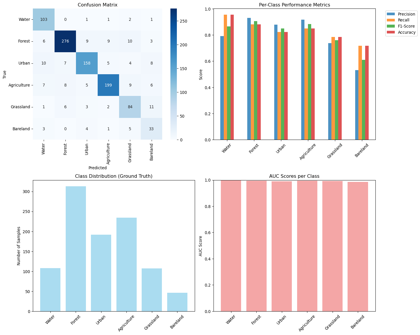
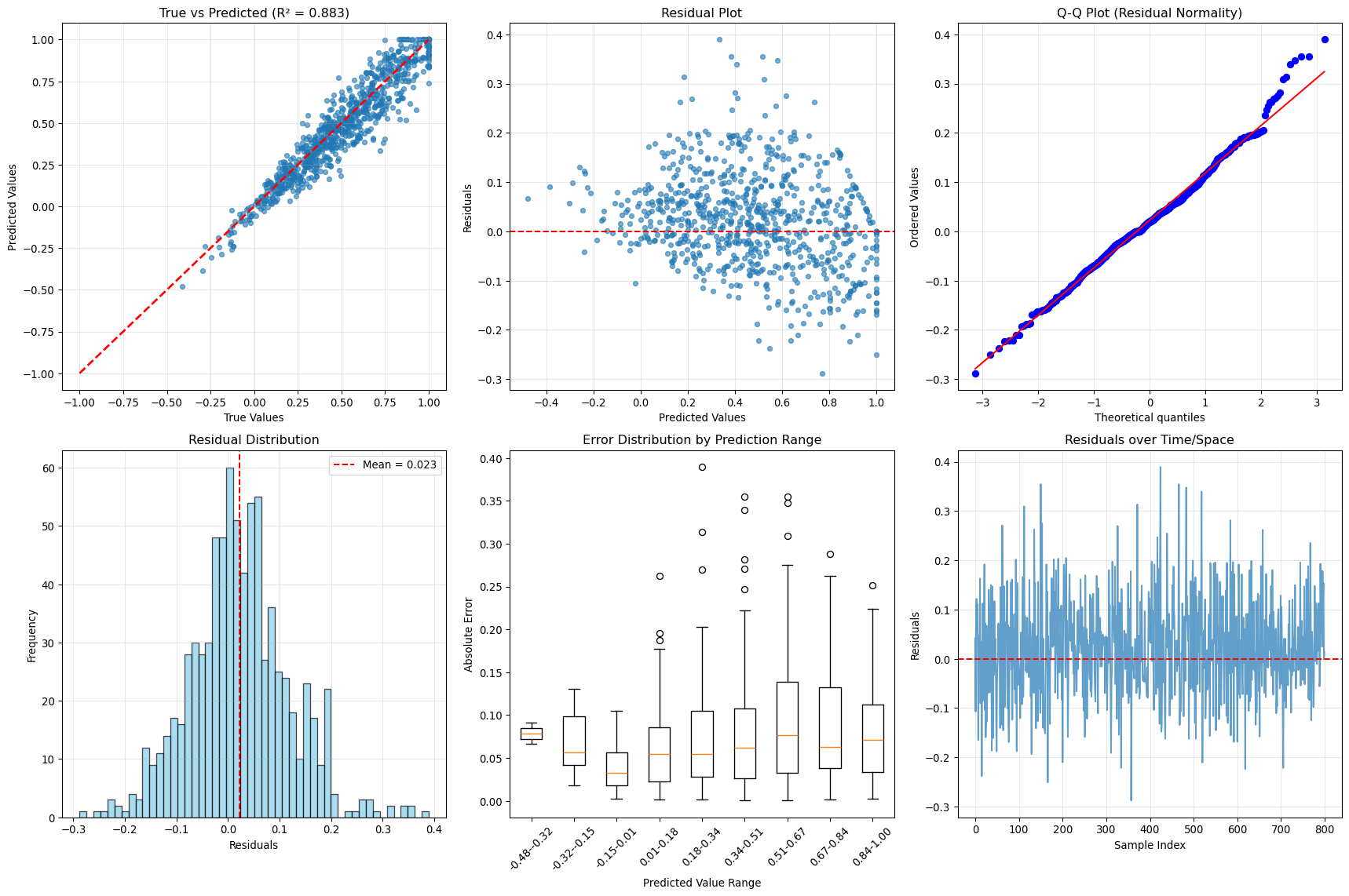
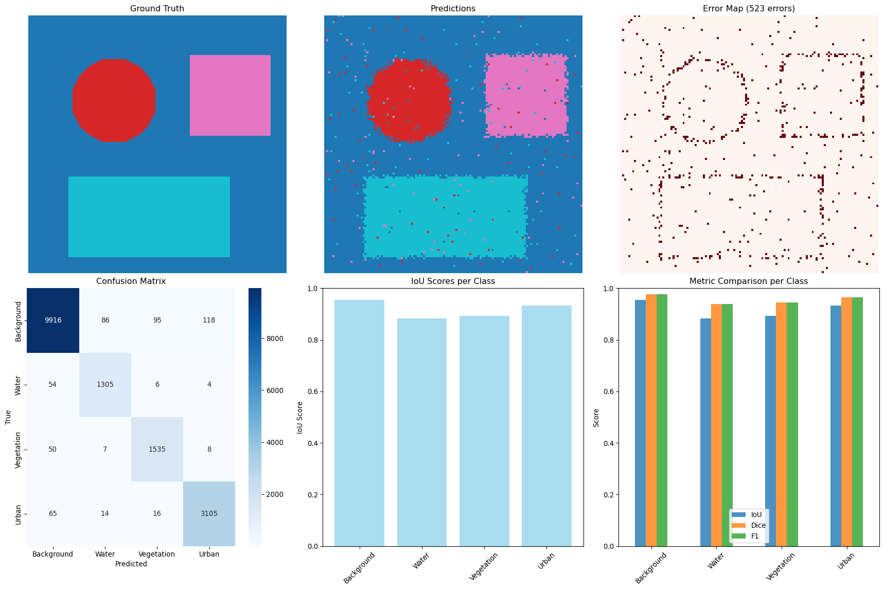
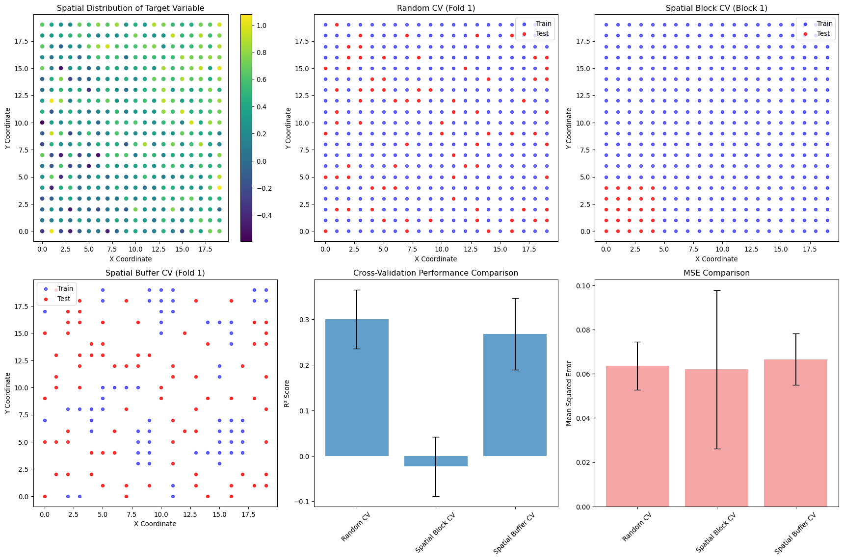
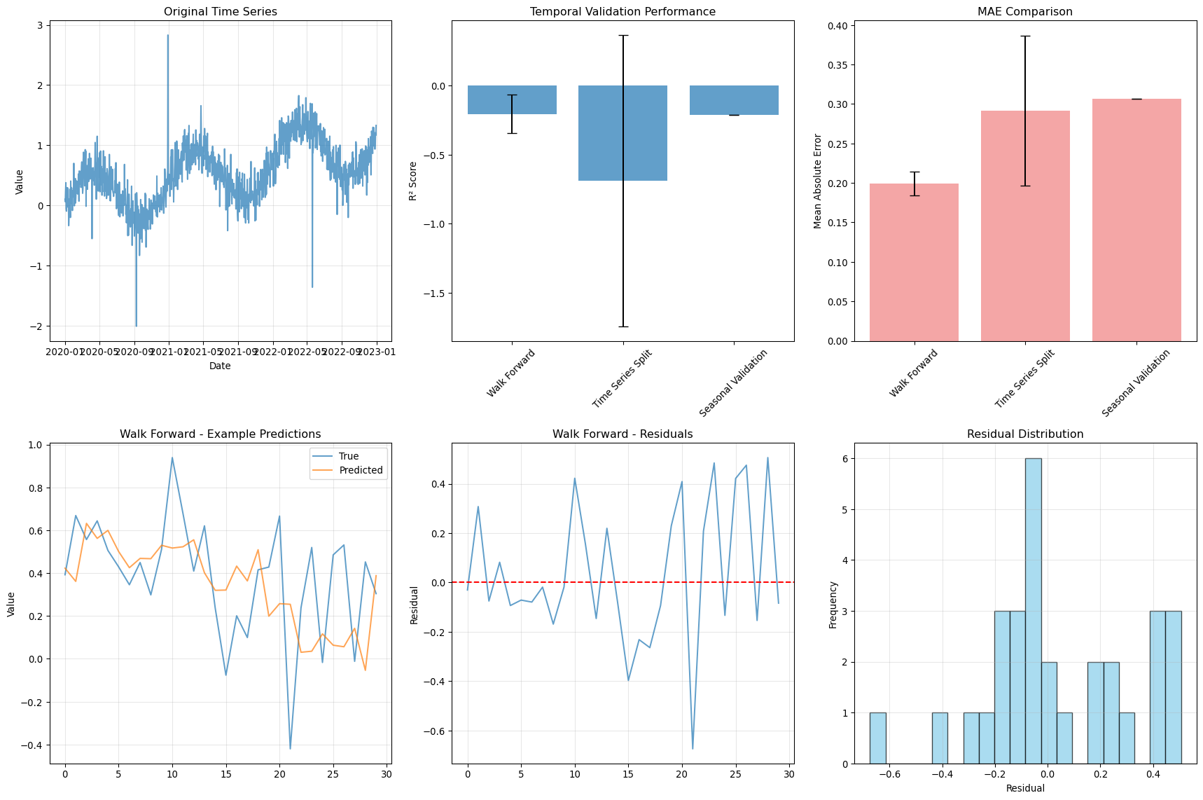
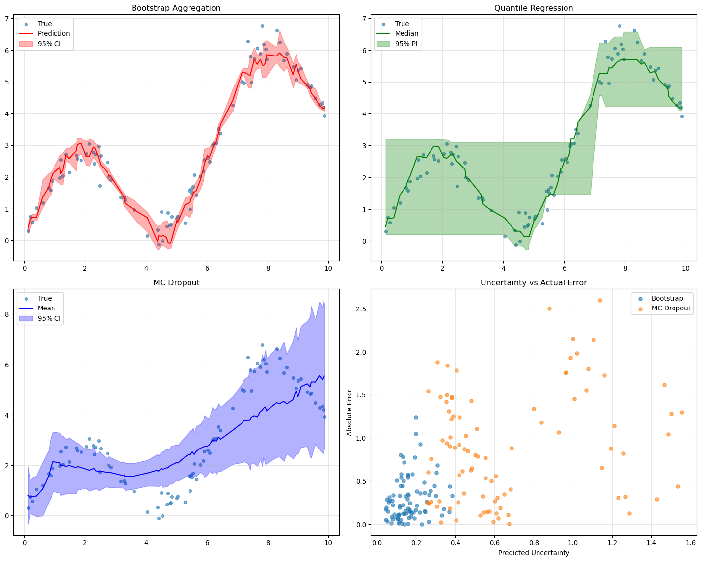
--- title: "Model Evaluation & Validation" subtitle: "Comprehensive evaluation strategies for geospatial models" jupyter: geoai format: html: code-fold: false --- ## Introduction to Model Evaluation ```{python} import torchimport torch.nn as nnimport numpy as npimport matplotlib.pyplot as pltimport pandas as pdfrom sklearn.metrics import accuracy_score, precision_recall_fscore_support, confusion_matrixfrom sklearn.metrics import mean_squared_error, mean_absolute_error, r2_scoreimport seaborn as snsfrom scipy import statsfrom sklearn.model_selection import train_test_splitprint (f"PyTorch version: { torch. __version__} " )``` ## Evaluation Metrics for Different Task Types ### Classification Metrics ```{python} def comprehensive_classification_evaluation():"""Demonstrate comprehensive classification evaluation metrics""" # Simulate classification results for land cover classification 42 )= 1000 = 6 = ['Water' , 'Forest' , 'Urban' , 'Agriculture' , 'Grassland' , 'Bareland' ]# Generate realistic predictions (imbalanced classes) = [0.1 , 0.3 , 0.2 , 0.25 , 0.1 , 0.05 ] # Different class frequencies = np.random.choice(num_classes, size= num_samples, p= class_probs)# Generate predictions with class-dependent accuracy = y_true.copy()= [0.95 , 0.88 , 0.82 , 0.85 , 0.78 , 0.70 ] # Different per-class accuracies for i in range (num_classes):= y_true == i= class_mask.sum ()= int (num_class_samples * (1 - class_accuracies[i]))if num_errors > 0 := np.random.choice(np.where(class_mask)[0 ], num_errors, replace= False )# Create confusion: assign to other classes = [j for j in range (num_classes) if j != i]= np.random.choice(other_classes, num_errors)# Generate prediction probabilities = np.zeros((num_samples, num_classes))for i in range (num_samples):# Create realistic probability distributions = y_true[i]= y_pred[i]# Base probabilities = np.random.dirichlet([0.5 ] * num_classes)# Boost true class probability += 0.5 # If prediction is correct, boost predicted class if true_class == pred_class:+= 0.3 # Normalize = base_probs / base_probs.sum ()# Calculate comprehensive metrics from sklearn.metrics import (accuracy_score, precision_recall_fscore_support, # Basic metrics = accuracy_score(y_true, y_pred)= precision_recall_fscore_support(y_true, y_pred, average= None )= precision_recall_fscore_support(y_true, y_pred, average= 'macro' )= precision_recall_fscore_support(y_true, y_pred, average= 'weighted' )# Confusion matrix = confusion_matrix(y_true, y_pred)# Per-class accuracy = cm.diagonal() / cm.sum (axis= 1 )# Multiclass AUC (one-vs-rest) = []for i in range (num_classes):= (y_true == i).astype(int )= roc_auc_score(y_true_binary, y_probs[:, i])print ("Classification Evaluation Results:" )print ("=" * 50 )print (f"Overall Accuracy: { accuracy:.3f} " )print (f"Macro F1-Score: { macro_f1:.3f} " )print (f"Weighted F1-Score: { weighted_f1:.3f} " )print (" \n Per-Class Metrics:" )print ("-" * 80 )print (f" { 'Class' :<12} { 'Precision' :<10} { 'Recall' :<10} { 'F1-Score' :<10} { 'Accuracy' :<10} { 'AUC' :<10} { 'Support' :<10} " )print ("-" * 80 )for i, class_name in enumerate (class_names):print (f" { class_name:<12} { precision[i]:<10.3f} { recall[i]:<10.3f} { f1[i]:<10.3f} { per_class_accuracy[i]:<10.3f} { auc_scores[i]:<10.3f} { support[i]:<10.0f} " )# Visualizations = plt.subplots(2 , 2 , figsize= (15 , 12 ))# Confusion Matrix = True , fmt= 'd' , cmap= 'Blues' , = class_names, yticklabels= class_names, ax= axes[0 ,0 ])0 ,0 ].set_title('Confusion Matrix' )0 ,0 ].set_xlabel('Predicted' )0 ,0 ].set_ylabel('True' )# Per-class metrics = pd.DataFrame({'Precision' : precision,'Recall' : recall,'F1-Score' : f1,'Accuracy' : per_class_accuracy= class_names)= 'bar' , ax= axes[0 ,1 ], alpha= 0.8 )0 ,1 ].set_title('Per-Class Performance Metrics' )0 ,1 ].set_ylabel('Score' )0 ,1 ].tick_params(axis= 'x' , rotation= 45 )0 ,1 ].legend(bbox_to_anchor= (1.05 , 1 ), loc= 'upper left' )# Class distribution = np.unique(y_true, return_counts= True )1 ,0 ].bar(class_names, counts, color= 'skyblue' , alpha= 0.7 )1 ,0 ].set_title('Class Distribution (Ground Truth)' )1 ,0 ].set_ylabel('Number of Samples' )1 ,0 ].tick_params(axis= 'x' , rotation= 45 )# AUC scores 1 ,1 ].bar(class_names, auc_scores, color= 'lightcoral' , alpha= 0.7 )1 ,1 ].set_title('AUC Scores per Class' )1 ,1 ].set_ylabel('AUC Score' )1 ,1 ].tick_params(axis= 'x' , rotation= 45 )1 ,1 ].set_ylim(0 , 1 )return {'accuracy' : accuracy,'precision' : precision,'recall' : recall,'f1' : f1,'confusion_matrix' : cm,'auc_scores' : auc_scores,'y_true' : y_true,'y_pred' : y_pred,'y_probs' : y_probs= comprehensive_classification_evaluation()``` ### Regression Metrics ```{python} def comprehensive_regression_evaluation():"""Demonstrate comprehensive regression evaluation metrics""" # Simulate regression results for vegetation index prediction 42 )= 800 # Generate realistic NDVI values (target) # Simulate seasonal pattern with spatial variation = np.sin(np.linspace(0 , 4 * np.pi, num_samples)) * 0.3 = np.random.normal(0 , 0.2 , num_samples)= np.random.normal(0 , 0.1 , num_samples)= 0.5 + time_component + spatial_component + noise= np.clip(y_true, - 1 , 1 ) # NDVI range # Generate predictions with realistic errors # Add heteroscedastic noise (error depends on true value) = np.random.normal(0 , 0.05 + 0.1 * np.abs (y_true))= - 0.02 # Slight systematic bias = y_true + prediction_noise + bias= np.clip(y_pred, - 1 , 1 )# Calculate comprehensive regression metrics = mean_absolute_error(y_true, y_pred)= mean_squared_error(y_true, y_pred)= np.sqrt(mse)= r2_score(y_true, y_pred)# Additional metrics def mean_absolute_percentage_error(y_true, y_pred):"""Calculate MAPE, handling near-zero values""" = np.abs (y_true) > 1e-6 return np.mean(np.abs ((y_true[mask] - y_pred[mask]) / y_true[mask])) * 100 def symmetric_mean_absolute_percentage_error(y_true, y_pred):"""Calculate symmetric MAPE""" return np.mean(2 * np.abs (y_true - y_pred) / (np.abs (y_true) + np.abs (y_pred))) * 100 = mean_absolute_percentage_error(y_true, y_pred)= symmetric_mean_absolute_percentage_error(y_true, y_pred)# Residual analysis = y_true - y_pred# Statistical tests # Shapiro-Wilk test for normality of residuals = stats.shapiro(residuals[:100 ]) # Sample for computational efficiency # Durbin-Watson test for autocorrelation (simplified) def durbin_watson(residuals):"""Calculate Durbin-Watson statistic""" = np.diff(residuals)return np.sum (diff** 2 ) / np.sum (residuals** 2 )= durbin_watson(residuals)# Quantile-based metrics = np.percentile(np.abs (residuals), 25 )= np.median(np.abs (residuals))= np.percentile(np.abs (residuals), 75 )= np.percentile(np.abs (residuals), 95 )print ("Regression Evaluation Results:" )print ("=" * 50 )print (f"Mean Absolute Error (MAE): { mae:.4f} " )print (f"Mean Squared Error (MSE): { mse:.4f} " )print (f"Root Mean Squared Error (RMSE): { rmse:.4f} " )print (f"R² Score: { r2:.4f} " )print (f"Mean Absolute Percentage Error (MAPE): { mape:.2f} %" )print (f"Symmetric MAPE: { smape:.2f} %" )print (" \n Residual Analysis:" )print (f"Mean Residual (Bias): { residuals. mean():.4f} " )print (f"Std of Residuals: { residuals. std():.4f} " )print (f"Residual Skewness: { stats. skew(residuals):.4f} " )print (f"Residual Kurtosis: { stats. kurtosis(residuals):.4f} " )print (f"Shapiro-Wilk p-value: { shapiro_p:.4f} " )print (f"Durbin-Watson statistic: { dw_stat:.4f} " )print (" \n Quantile-based Error Analysis:" )print (f"25th percentile error: { q25_error:.4f} " )print (f"Median error: { median_error:.4f} " )print (f"75th percentile error: { q75_error:.4f} " )print (f"95th percentile error: { q95_error:.4f} " )# Visualizations = plt.subplots(2 , 3 , figsize= (18 , 12 ))# Scatter plot: True vs Predicted 0 ,0 ].scatter(y_true, y_pred, alpha= 0.6 , s= 20 )0 ,0 ].plot([- 1 , 1 ], [- 1 , 1 ], 'r--' , lw= 2 ) # Perfect prediction line 0 ,0 ].set_xlabel('True Values' )0 ,0 ].set_ylabel('Predicted Values' )0 ,0 ].set_title(f'True vs Predicted (R² = { r2:.3f} )' )0 ,0 ].grid(True , alpha= 0.3 )# Residual plot 0 ,1 ].scatter(y_pred, residuals, alpha= 0.6 , s= 20 )0 ,1 ].axhline(y= 0 , color= 'r' , linestyle= '--' )0 ,1 ].set_xlabel('Predicted Values' )0 ,1 ].set_ylabel('Residuals' )0 ,1 ].set_title('Residual Plot' )0 ,1 ].grid(True , alpha= 0.3 )# Q-Q plot for residual normality = "norm" , plot= axes[0 ,2 ])0 ,2 ].set_title('Q-Q Plot (Residual Normality)' )0 ,2 ].grid(True , alpha= 0.3 )# Residual histogram 1 ,0 ].hist(residuals, bins= 50 , alpha= 0.7 , color= 'skyblue' , edgecolor= 'black' )1 ,0 ].axvline(residuals.mean(), color= 'red' , linestyle= '--' , label= f'Mean = { residuals. mean():.3f} ' )1 ,0 ].set_xlabel('Residuals' )1 ,0 ].set_ylabel('Frequency' )1 ,0 ].set_title('Residual Distribution' )1 ,0 ].legend()1 ,0 ].grid(True , alpha= 0.3 )# Error distribution by predicted value ranges = np.linspace(y_pred.min (), y_pred.max (), 10 )= []= []for i in range (len (pred_ranges)- 1 ):= (y_pred >= pred_ranges[i]) & (y_pred < pred_ranges[i+ 1 ])if mask.sum () > 0 :abs (residuals[mask]))f' { pred_ranges[i]:.2f} - { pred_ranges[i+ 1 ]:.2f} ' )1 ,1 ].boxplot(range_errors, labels= range_labels)1 ,1 ].set_xlabel('Predicted Value Range' )1 ,1 ].set_ylabel('Absolute Error' )1 ,1 ].set_title('Error Distribution by Prediction Range' )1 ,1 ].tick_params(axis= 'x' , rotation= 45 )# Time series of residuals (if applicable) 1 ,2 ].plot(residuals, alpha= 0.7 )1 ,2 ].axhline(y= 0 , color= 'r' , linestyle= '--' )1 ,2 ].set_xlabel('Sample Index' )1 ,2 ].set_ylabel('Residuals' )1 ,2 ].set_title('Residuals over Time/Space' )1 ,2 ].grid(True , alpha= 0.3 )return {'mae' : mae, 'mse' : mse, 'rmse' : rmse, 'r2' : r2,'mape' : mape, 'smape' : smape,'residuals' : residuals,'y_true' : y_true, 'y_pred' : y_pred= comprehensive_regression_evaluation()``` ### Segmentation Metrics ```{python} def comprehensive_segmentation_evaluation():"""Demonstrate comprehensive segmentation evaluation metrics""" # Simulate segmentation results 42 )= 128 , 128 = 4 = ['Background' , 'Water' , 'Vegetation' , 'Urban' ]# Generate realistic ground truth segmentation mask = np.zeros((height, width), dtype= int )# Create regions for different classes # Water body (circular) = width// 3 , height// 3 = np.ogrid[:height, :width]= (x_indices - center_x)** 2 + (y_indices - center_y)** 2 < (width// 6 )** 2 = 1 # Vegetation (upper right) 20 :60 , 80 :120 ] = 2 # Urban (lower region) 80 :120 , 20 :100 ] = 3 # Generate predictions with realistic errors = y_true.copy()# Add boundary errors from scipy import ndimage= ndimage.binary_dilation(ndimage.laplace(y_true) != 0 )# Randomly flip some edge pixels = np.where(edges)= len (edge_indices[0 ]) // 4 = np.random.choice(len (edge_indices[0 ]), num_edge_errors, replace= False )for idx in error_indices:= edge_indices[0 ][idx], edge_indices[1 ][idx]# Assign to random neighboring class = [y_true[max (0 ,y- 1 ):min (height,y+ 2 ), max (0 ,x- 1 ):min (width,x+ 2 )]]= np.unique(neighbors)= [c for c in unique_neighbors if c != y_true[y, x]]if other_classes:= np.random.choice(other_classes)# Add some random noise = (height * width) // 50 = np.random.randint(0 , height, num_random_errors)= np.random.randint(0 , width, num_random_errors)for y, x in zip (error_y, error_x):= np.random.randint(0 , num_classes)# Calculate segmentation metrics def calculate_segmentation_metrics(y_true, y_pred, num_classes):"""Calculate comprehensive segmentation metrics""" # Flatten arrays = y_true.flatten()= y_pred.flatten()# Basic accuracy = accuracy_score(y_true_flat, y_pred_flat)# Per-class metrics = precision_recall_fscore_support(= None , zero_division= 0 # Confusion matrix = confusion_matrix(y_true_flat, y_pred_flat)# IoU (Intersection over Union) per class = []= []for i in range (num_classes):# True positives, false positives, false negatives = cm[i, i]= cm[:, i].sum () - tp= cm[i, :].sum () - tp# IoU = tp / (tp + fp + fn) if (tp + fp + fn) > 0 else 0 # Dice coefficient = 2 * tp / (2 * tp + fp + fn) if (2 * tp + fp + fn) > 0 else 0 # Mean IoU = np.mean(iou_scores)# Pixel accuracy (same as overall accuracy) = accuracy# Mean accuracy (average of per-class accuracies) = cm.diagonal() / cm.sum (axis= 1 )= np.mean(class_accuracies)# Frequency weighted IoU = cm.sum (axis= 1 ) / cm.sum ()= np.sum (class_frequencies * iou_scores)return {'pixel_accuracy' : pixel_accuracy,'mean_accuracy' : mean_accuracy,'mean_iou' : mean_iou,'freq_weighted_iou' : freq_weighted_iou,'iou_scores' : iou_scores,'dice_scores' : dice_scores,'precision' : precision,'recall' : recall,'f1' : f1,'confusion_matrix' : cm= calculate_segmentation_metrics(y_true, y_pred, num_classes)print ("Segmentation Evaluation Results:" )print ("=" * 50 )print (f"Pixel Accuracy: { metrics['pixel_accuracy' ]:.4f} " )print (f"Mean Accuracy: { metrics['mean_accuracy' ]:.4f} " )print (f"Mean IoU: { metrics['mean_iou' ]:.4f} " )print (f"Frequency Weighted IoU: { metrics['freq_weighted_iou' ]:.4f} " )print (" \n Per-Class Metrics:" )print ("-" * 70 )print (f" { 'Class' :<12} { 'IoU' :<8} { 'Dice' :<8} { 'Precision' :<10} { 'Recall' :<10} { 'F1' :<8} " )print ("-" * 70 )for i, class_name in enumerate (class_names):print (f" { class_name:<12} { metrics['iou_scores' ][i]:<8.3f} { metrics['dice_scores' ][i]:<8.3f} " f" { metrics['precision' ][i]:<10.3f} { metrics['recall' ][i]:<10.3f} { metrics['f1' ][i]:<8.3f} " )# Visualizations = plt.subplots(2 , 3 , figsize= (18 , 12 ))# Ground truth = axes[0 ,0 ].imshow(y_true, cmap= 'tab10' , vmin= 0 , vmax= num_classes- 1 )0 ,0 ].set_title('Ground Truth' )0 ,0 ].axis('off' )# Predictions = axes[0 ,1 ].imshow(y_pred, cmap= 'tab10' , vmin= 0 , vmax= num_classes- 1 )0 ,1 ].set_title('Predictions' )0 ,1 ].axis('off' )# Error map = (y_true != y_pred).astype(int )0 ,2 ].imshow(error_map, cmap= 'Reds' )0 ,2 ].set_title(f'Error Map ( { error_map. sum ()} errors)' )0 ,2 ].axis('off' )# Confusion matrix 'confusion_matrix' ], annot= True , fmt= 'd' , cmap= 'Blues' ,= class_names, yticklabels= class_names, ax= axes[1 ,0 ])1 ,0 ].set_title('Confusion Matrix' )1 ,0 ].set_xlabel('Predicted' )1 ,0 ].set_ylabel('True' )# Per-class IoU 1 ,1 ].bar(class_names, metrics['iou_scores' ], color= 'skyblue' , alpha= 0.7 )1 ,1 ].set_title('IoU Scores per Class' )1 ,1 ].set_ylabel('IoU Score' )1 ,1 ].tick_params(axis= 'x' , rotation= 45 )1 ,1 ].set_ylim(0 , 1 )# Metrics comparison = pd.DataFrame({'IoU' : metrics['iou_scores' ],'Dice' : metrics['dice_scores' ],'F1' : metrics['f1' ]= class_names)= 'bar' , ax= axes[1 ,2 ], alpha= 0.8 )1 ,2 ].set_title('Metric Comparison per Class' )1 ,2 ].set_ylabel('Score' )1 ,2 ].tick_params(axis= 'x' , rotation= 45 )1 ,2 ].legend()1 ,2 ].set_ylim(0 , 1 )return metrics, y_true, y_pred= comprehensive_segmentation_evaluation()``` ## Spatial Validation Strategies ### Cross-Validation with Spatial Awareness ```{python} def demonstrate_spatial_cross_validation():"""Demonstrate spatial cross-validation strategies""" # Simulate spatial data with coordinates 42 )# Generate spatial grid = 20 = np.repeat(np.arange(grid_size), grid_size)= np.tile(np.arange(grid_size), grid_size)= len (x_coords)# Generate spatially correlated features and target # Create spatial autocorrelation structure def spatial_correlation(x1, y1, x2, y2, correlation_range= 5 ):"""Calculate spatial correlation based on distance""" = np.sqrt((x1 - x2)** 2 + (y1 - y2)** 2 )return np.exp(- distance / correlation_range)# Generate correlated target variable = np.zeros(n_samples)= 0.5 * (x_coords / grid_size) + 0.3 * (y_coords / grid_size)for i in range (n_samples):# Add spatially correlated noise = 0 for j in range (min (50 , n_samples)): # Limit for computational efficiency if i != j:= spatial_correlation(x_coords[i], y_coords[i], x_coords[j], y_coords[j])+= weight * np.random.normal(0 , 0.1 )= base_trend[i] + spatial_component + np.random.normal(0 , 0.2 )# Generate features = np.column_stack([/ grid_size, # Normalized x coordinate / grid_size, # Normalized y coordinate 0 , 1 , n_samples), # Random feature 1 0 , 1 , n_samples), # Random feature 2 # Different cross-validation strategies def random_cv_split(X, y, n_folds= 5 ):"""Standard random cross-validation""" from sklearn.model_selection import KFold= KFold(n_splits= n_folds, shuffle= True , random_state= 42 )return list (kfold.split(X))def spatial_block_cv_split(x_coords, y_coords, n_blocks= 4 ):"""Spatial block cross-validation""" # Divide space into blocks = np.linspace(x_coords.min (), x_coords.max (), int (np.sqrt(n_blocks))+ 1 )= np.linspace(y_coords.min (), y_coords.max (), int (np.sqrt(n_blocks))+ 1 )= []for i in range (len (x_blocks)- 1 ):for j in range (len (y_blocks)- 1 ):# Test block = ((x_coords >= x_blocks[i]) & (x_coords < x_blocks[i+ 1 ]) & >= y_blocks[j]) & (y_coords < y_blocks[j+ 1 ]))# Training set is everything else = ~ test_maskif test_mask.sum () > 0 and train_mask.sum () > 0 := np.where(train_mask)[0 ]= np.where(test_mask)[0 ]return foldsdef spatial_buffer_cv_split(x_coords, y_coords, n_folds= 5 , buffer_distance= 2 ):"""Spatial cross-validation with buffer zones""" from sklearn.model_selection import KFold# First, get random splits = KFold(n_splits= n_folds, shuffle= True , random_state= 42 )= list (kfold.split(range (len (x_coords))))= []for train_idx, test_idx in random_splits:# Remove training samples too close to test samples = []for train_i in train_idx:= float ('inf' )for test_i in test_idx:= np.sqrt((x_coords[train_i] - x_coords[test_i])** 2 + - y_coords[test_i])** 2 )= min (min_dist_to_test, dist)if min_dist_to_test >= buffer_distance:if len (filtered_train_idx) > 0 :return buffered_splits# Evaluate different CV strategies from sklearn.linear_model import LinearRegressionfrom sklearn.metrics import mean_squared_error, r2_scoredef evaluate_cv_strategy(X, y, cv_splits, strategy_name):"""Evaluate a cross-validation strategy""" = []= []for fold, (train_idx, test_idx) in enumerate (cv_splits):# Train model = LinearRegression()# Predict on test set = model.predict(X[test_idx])# Calculate metrics = r2_score(y[test_idx], y_pred)= mean_squared_error(y[test_idx], y_pred)return {'strategy' : strategy_name,'r2_mean' : np.mean(r2_scores),'r2_std' : np.std(r2_scores),'mse_mean' : np.mean(mse_scores),'mse_std' : np.std(mse_scores),'n_folds' : len (cv_splits)# Apply different CV strategies = random_cv_split(X, y, n_folds= 5 )= spatial_block_cv_split(x_coords, y_coords, n_blocks= 16 )= spatial_buffer_cv_split(x_coords, y_coords, n_folds= 5 , buffer_distance= 2 )# Evaluate strategies = []'Random CV' ))'Spatial Block CV' ))'Spatial Buffer CV' ))# Display results print ("Spatial Cross-Validation Comparison:" )print ("=" * 60 )print (f" { 'Strategy' :<20} { 'R² Mean' :<10} { 'R² Std' :<10} { 'MSE Mean' :<10} { 'MSE Std' :<10} { 'Folds' :<6} " )print ("-" * 60 )for result in results:print (f" { result['strategy' ]:<20} { result['r2_mean' ]:<10.3f} { result['r2_std' ]:<10.3f} " f" { result['mse_mean' ]:<10.3f} { result['mse_std' ]:<10.3f} { result['n_folds' ]:<6} " )# Visualizations = plt.subplots(2 , 3 , figsize= (18 , 12 ))# Data distribution = axes[0 ,0 ].scatter(x_coords, y_coords, c= y, cmap= 'viridis' , s= 30 )0 ,0 ].set_title('Spatial Distribution of Target Variable' )0 ,0 ].set_xlabel('X Coordinate' )0 ,0 ].set_ylabel('Y Coordinate' )= axes[0 ,0 ])# Random CV example (first fold) = random_splits[0 ]0 ,1 ].scatter(x_coords[train_idx], y_coords[train_idx], c= 'blue' , s= 20 , alpha= 0.6 , label= 'Train' )0 ,1 ].scatter(x_coords[test_idx], y_coords[test_idx], c= 'red' , s= 20 , alpha= 0.8 , label= 'Test' )0 ,1 ].set_title('Random CV (Fold 1)' )0 ,1 ].set_xlabel('X Coordinate' )0 ,1 ].set_ylabel('Y Coordinate' )0 ,1 ].legend()# Block CV example (first fold) if block_splits:= block_splits[0 ]0 ,2 ].scatter(x_coords[train_idx], y_coords[train_idx], c= 'blue' , s= 20 , alpha= 0.6 , label= 'Train' )0 ,2 ].scatter(x_coords[test_idx], y_coords[test_idx], c= 'red' , s= 20 , alpha= 0.8 , label= 'Test' )0 ,2 ].set_title('Spatial Block CV (Block 1)' )0 ,2 ].set_xlabel('X Coordinate' )0 ,2 ].set_ylabel('Y Coordinate' )0 ,2 ].legend()# Buffer CV example (first fold) if buffer_splits:= buffer_splits[0 ]1 ,0 ].scatter(x_coords[train_idx], y_coords[train_idx], c= 'blue' , s= 20 , alpha= 0.6 , label= 'Train' )1 ,0 ].scatter(x_coords[test_idx], y_coords[test_idx], c= 'red' , s= 20 , alpha= 0.8 , label= 'Test' )1 ,0 ].set_title('Spatial Buffer CV (Fold 1)' )1 ,0 ].set_xlabel('X Coordinate' )1 ,0 ].set_ylabel('Y Coordinate' )1 ,0 ].legend()# Performance comparison = [r['strategy' ] for r in results]= [r['r2_mean' ] for r in results]= [r['r2_std' ] for r in results]= axes[1 ,1 ].bar(strategies, r2_means, yerr= r2_stds, capsize= 5 , alpha= 0.7 )1 ,1 ].set_title('Cross-Validation Performance Comparison' )1 ,1 ].set_ylabel('R² Score' )1 ,1 ].tick_params(axis= 'x' , rotation= 45 )# MSE comparison = [r['mse_mean' ] for r in results]= [r['mse_std' ] for r in results]= axes[1 ,2 ].bar(strategies, mse_means, yerr= mse_stds, capsize= 5 , alpha= 0.7 , color= 'lightcoral' )1 ,2 ].set_title('MSE Comparison' )1 ,2 ].set_ylabel('Mean Squared Error' )1 ,2 ].tick_params(axis= 'x' , rotation= 45 )return results, X, y, x_coords, y_coords= demonstrate_spatial_cross_validation()``` ## Temporal Validation ### Time Series Cross-Validation ```{python} def demonstrate_temporal_validation():"""Demonstrate temporal validation strategies for time series data""" # Generate temporal dataset 42 )# Create time series with trend, seasonality, and noise = 365 * 3 # 3 years of daily data = pd.date_range('2020-01-01' , periods= n_timesteps, freq= 'D' )# Generate synthetic time series = np.arange(n_timesteps)# Trend component = 0.001 * t# Seasonal components = 0.5 * np.sin(2 * np.pi * t / 365 )= 0.1 * np.sin(2 * np.pi * t / 7 )# Random noise = np.random.normal(0 , 0.2 , n_timesteps)# Combine components = trend + annual_cycle + weekly_cycle + noise# Add some extreme events = np.random.choice(n_timesteps, 10 , replace= False )+= np.random.normal(0 , 2 , 10 )# Create features (lagged values, moving averages, etc.) def create_temporal_features(y, lookback_window= 30 ):"""Create temporal features for time series prediction""" = []= []for i in range (lookback_window, len (y)):# Lagged values = y[i- lookback_window:i]# Statistical features = [min (lag_features),max (lag_features),- 1 ], # Most recent value - 7 ] # Value from a week ago # Time features = (i % 365 ) / 365 = (i % 7 ) / 7 # Combine all features = list (lag_features) + stat_features + [day_of_year, day_of_week]return np.array(features), np.array(targets)= create_temporal_features(y, lookback_window= 7 )# Temporal validation strategies def walk_forward_validation(X, y, n_splits= 5 , test_size= 30 ):"""Walk-forward (expanding window) validation""" = len (X)= n_samples // 2 = []for i in range (n_splits):# Expanding training set = min_train_size + i * test_size= train_end= min (test_start + test_size, n_samples)if test_end > test_start:= np.arange(0 , train_end)= np.arange(test_start, test_end)return splitsdef time_series_split_validation(X, y, n_splits= 5 ):"""Time series split validation (rolling window)""" from sklearn.model_selection import TimeSeriesSplit= TimeSeriesSplit(n_splits= n_splits)return list (tss.split(X))def seasonal_validation(X, y, season_length= 365 ):"""Seasonal validation - train on some seasons, test on others""" = len (X)= n_samples // season_length= []for test_season in range (1 , n_seasons): # Skip first season for training # Training: all seasons except test season = []for season in range (n_seasons):if season != test_season:= season * season_length= min ((season + 1 ) * season_length, n_samples)range (season_start, season_end))# Test: specific season = test_season * season_length= min ((test_season + 1 ) * season_length, n_samples)= list (range (test_start, test_end))if len (train_idx) > 0 and len (test_idx) > 0 :return splits# Evaluate different temporal validation strategies from sklearn.ensemble import RandomForestRegressordef evaluate_temporal_strategy(X, y, cv_splits, strategy_name):"""Evaluate temporal validation strategy""" = []= []= []for fold, (train_idx, test_idx) in enumerate (cv_splits):# Train model = RandomForestRegressor(n_estimators= 50 , random_state= 42 )# Predict = model.predict(X[test_idx])# Metrics = r2_score(y[test_idx], y_pred)= mean_absolute_error(y[test_idx], y_pred)return {'strategy' : strategy_name,'r2_mean' : np.mean(r2_scores),'r2_std' : np.std(r2_scores),'mae_mean' : np.mean(mae_scores),'mae_std' : np.std(mae_scores),'predictions' : predictions_all,'n_folds' : len (cv_splits)# Apply different strategies = walk_forward_validation(X, y_target, n_splits= 5 )= time_series_split_validation(X, y_target, n_splits= 5 )= seasonal_validation(X, y_target, season_length= 365 )# Evaluate strategies = []'Walk Forward' ))'Time Series Split' ))'Seasonal Validation' ))# Display results print ("Temporal Validation Comparison:" )print ("=" * 60 )print (f" { 'Strategy' :<20} { 'R² Mean' :<10} { 'R² Std' :<10} { 'MAE Mean' :<10} { 'MAE Std' :<10} { 'Folds' :<6} " )print ("-" * 60 )for result in temporal_results:print (f" { result['strategy' ]:<20} { result['r2_mean' ]:<10.3f} { result['r2_std' ]:<10.3f} " f" { result['mae_mean' ]:<10.3f} { result['mae_std' ]:<10.3f} { result['n_folds' ]:<6} " )# Visualizations = plt.subplots(2 , 3 , figsize= (18 , 12 ))# Original time series 0 ,0 ].plot(time_index[:len (y)], y, alpha= 0.7 )0 ,0 ].set_title('Original Time Series' )0 ,0 ].set_xlabel('Date' )0 ,0 ].set_ylabel('Value' )0 ,0 ].grid(True , alpha= 0.3 )# Performance comparison = [r['strategy' ] for r in temporal_results]= [r['r2_mean' ] for r in temporal_results]= [r['r2_std' ] for r in temporal_results]= axes[0 ,1 ].bar(strategies, r2_means, yerr= r2_stds, capsize= 5 , alpha= 0.7 )0 ,1 ].set_title('Temporal Validation Performance' )0 ,1 ].set_ylabel('R² Score' )0 ,1 ].tick_params(axis= 'x' , rotation= 45 )# MAE comparison = [r['mae_mean' ] for r in temporal_results]= [r['mae_std' ] for r in temporal_results]= axes[0 ,2 ].bar(strategies, mae_means, yerr= mae_stds, capsize= 5 , alpha= 0.7 , color= 'lightcoral' )0 ,2 ].set_title('MAE Comparison' )0 ,2 ].set_ylabel('Mean Absolute Error' )0 ,2 ].tick_params(axis= 'x' , rotation= 45 )# Example predictions for first strategy only (to fit in 2x3 grid) if temporal_results:= temporal_results[0 ] # Show only first strategy = result['predictions' ][0 ]1 ,0 ].plot(y_true_fold, alpha= 0.7 , label= 'True' )1 ,0 ].plot(y_pred_fold, alpha= 0.7 , label= 'Predicted' )1 ,0 ].set_title(f' { result["strategy" ]} - Example Predictions' )1 ,0 ].set_ylabel('Value' )1 ,0 ].legend()1 ,0 ].grid(True , alpha= 0.3 )# Residuals for first strategy = y_true_fold - y_pred_fold1 ,1 ].plot(residuals, alpha= 0.7 )1 ,1 ].axhline(y= 0 , color= 'r' , linestyle= '--' )1 ,1 ].set_title(f' { result["strategy" ]} - Residuals' )1 ,1 ].set_ylabel('Residual' )1 ,1 ].grid(True , alpha= 0.3 )# Residual histogram 1 ,2 ].hist(residuals, bins= 20 , alpha= 0.7 , color= 'skyblue' , edgecolor= 'black' )1 ,2 ].set_title('Residual Distribution' )1 ,2 ].set_xlabel('Residual' )1 ,2 ].set_ylabel('Frequency' )1 ,2 ].grid(True , alpha= 0.3 )return temporal_results, X, y_target, time_index= demonstrate_temporal_validation()``` ## Model Uncertainty Quantification ### Uncertainty Estimation Methods ```{python} def demonstrate_uncertainty_quantification():"""Demonstrate uncertainty quantification methods""" # Generate dataset with varying noise levels 42 )= 300 = np.linspace(0 , 10 , n_samples).reshape(- 1 , 1 )# Create heteroscedastic data (varying uncertainty) = 0.1 + 0.3 * np.abs (np.sin(X.flatten()))= 2 * np.sin(X.flatten()) + 0.5 * X.flatten() + np.random.normal(0 , noise_levels)# Split data = np.random.choice(n_samples, int (0.7 * n_samples), replace= False )= np.setdiff1d(np.arange(n_samples), train_idx)= X[train_idx], X[test_idx]= y[train_idx], y[test_idx]# Method 1: Bootstrap Aggregation def bootstrap_uncertainty(X_train, y_train, X_test, n_bootstrap= 100 ):"""Estimate uncertainty using bootstrap aggregation""" from sklearn.ensemble import RandomForestRegressor= []for i in range (n_bootstrap):# Bootstrap sample = len (X_train)= np.random.choice(n_train, n_train, replace= True )= X_train[bootstrap_idx]= y_train[bootstrap_idx]# Train model = RandomForestRegressor(n_estimators= 20 , random_state= i)# Predict = model.predict(X_test)= np.array(predictions)# Calculate statistics = np.mean(predictions, axis= 0 )= np.std(predictions, axis= 0 )# Confidence intervals = np.percentile(predictions, 2.5 , axis= 0 )= np.percentile(predictions, 97.5 , axis= 0 )return mean_pred, std_pred, ci_lower, ci_upper# Method 2: Quantile Regression def quantile_regression_uncertainty(X_train, y_train, X_test, quantiles= [0.025 , 0.5 , 0.975 ]):"""Estimate uncertainty using quantile regression""" from sklearn.ensemble import GradientBoostingRegressor= {}for q in quantiles:= GradientBoostingRegressor(loss= 'quantile' , alpha= q, random_state= 42 )= model.predict(X_test)return predictions# Method 3: Monte Carlo Dropout (simplified) class MCDropoutModel(nn.Module):"""Simple neural network with Monte Carlo Dropout""" def __init__ (self , input_dim= 1 , hidden_dim= 50 , dropout_rate= 0.5 ):super ().__init__ ()self .layers = nn.Sequential(1 )self .dropout_rate = dropout_ratedef forward(self , x):return self .layers(x)def predict_with_uncertainty(self , x, n_samples= 100 ):"""Predict with MC Dropout uncertainty""" self .train() # Keep in training mode for dropout = []with torch.no_grad():for _ in range (n_samples):= self (x)= np.array(predictions).squeeze()if predictions.ndim == 1 : # Single prediction return predictions.mean(), predictions.std()else : # Multiple predictions return predictions.mean(axis= 0 ), predictions.std(axis= 0 )def mc_dropout_uncertainty(X_train, y_train, X_test):"""Train MC Dropout model and get uncertainty estimates""" # Convert to tensors = torch.FloatTensor(X_train)= torch.FloatTensor(y_train).unsqueeze(1 )= torch.FloatTensor(X_test)# Train model = MCDropoutModel()= torch.optim.Adam(model.parameters(), lr= 0.01 )= nn.MSELoss()# Simple training loop for epoch in range (200 ):= model(X_train_tensor)= criterion(outputs, y_train_tensor)# Get predictions with uncertainty = model.predict_with_uncertainty(X_test_tensor)return mean_pred, std_pred# Apply different uncertainty methods print ("Uncertainty Quantification Methods:" )print ("=" * 50 )# Bootstrap print ("Running Bootstrap Aggregation..." )= bootstrap_uncertainty(X_train, y_train, X_test)# Quantile regression print ("Running Quantile Regression..." )= quantile_regression_uncertainty(X_train, y_train, X_test)# MC Dropout print ("Running MC Dropout..." )= mc_dropout_uncertainty(X_train, y_train, X_test)# Calculate uncertainty metrics def evaluate_uncertainty(y_true, mean_pred, std_pred= None , ci_lower= None , ci_upper= None ):"""Evaluate uncertainty estimation quality""" # Prediction accuracy = mean_absolute_error(y_true, mean_pred)= np.sqrt(mean_squared_error(y_true, mean_pred))= r2_score(y_true, mean_pred)= {'mae' : mae, 'rmse' : rmse, 'r2' : r2}if std_pred is not None :# Uncertainty calibration = np.abs (y_true - mean_pred)# Correlation between predicted uncertainty and actual errors = np.corrcoef(std_pred, residuals)[0 , 1 ]'uncertainty_correlation' ] = uncertainty_correlationif ci_lower is not None and ci_upper is not None :# Coverage probability (should be ~95% for 95% CI) = (y_true >= ci_lower) & (y_true <= ci_upper)= np.mean(in_interval)'coverage' ] = coverage# Interval width = np.mean(ci_upper - ci_lower)'mean_interval_width' ] = interval_widthreturn metrics# Evaluate methods = evaluate_uncertainty(y_test, boot_mean, boot_std, boot_lower, boot_upper)= evaluate_uncertainty(y_test, quantile_preds[0.5 ], = quantile_preds[0.025 ], = quantile_preds[0.975 ])= evaluate_uncertainty(y_test, mc_mean, mc_std)print (" \n Uncertainty Evaluation Results:" )print ("-" * 60 )print (f" { 'Method' :<20} { 'MAE' :<8} { 'RMSE' :<8} { 'R²' :<8} { 'Coverage' :<10} { 'Uncert.Corr' :<12} " )print ("-" * 60 )= ['Bootstrap' , boot_metrics),'Quantile Reg.' , quantile_metrics),'MC Dropout' , mc_metrics)for method_name, metrics in methods_data:= metrics.get('coverage' , 0 )= metrics.get('uncertainty_correlation' , 0 )print (f" { method_name:<20} { metrics['mae' ]:<8.3f} { metrics['rmse' ]:<8.3f} { metrics['r2' ]:<8.3f} " f" { coverage:<10.3f} { uncert_corr:<12.3f} " )# Visualizations = plt.subplots(2 , 2 , figsize= (15 , 12 ))# Sort test data for plotting = np.argsort(X_test.flatten())= X_test[sort_idx]= y_test[sort_idx]# Bootstrap results 0 ,0 ].scatter(X_test, y_test, alpha= 0.6 , s= 20 , label= 'True' )0 ,0 ].plot(X_test_sorted, boot_mean[sort_idx], 'r-' , label= 'Prediction' )0 ,0 ].fill_between(X_test_sorted.flatten(), = 0.3 , color= 'red' , label= '95% CI' )0 ,0 ].set_title('Bootstrap Aggregation' )0 ,0 ].legend()0 ,0 ].grid(True , alpha= 0.3 )# Quantile regression 0 ,1 ].scatter(X_test, y_test, alpha= 0.6 , s= 20 , label= 'True' )0 ,1 ].plot(X_test_sorted, quantile_preds[0.5 ][sort_idx], 'g-' , label= 'Median' )0 ,1 ].fill_between(X_test_sorted.flatten(),0.025 ][sort_idx], quantile_preds[0.975 ][sort_idx],= 0.3 , color= 'green' , label= '95% PI' )0 ,1 ].set_title('Quantile Regression' )0 ,1 ].legend()0 ,1 ].grid(True , alpha= 0.3 )# MC Dropout 1 ,0 ].scatter(X_test, y_test, alpha= 0.6 , s= 20 , label= 'True' )1 ,0 ].plot(X_test_sorted, mc_mean[sort_idx], 'b-' , label= 'Mean' )# Calculate confidence intervals for MC Dropout = mc_mean - 1.96 * mc_std= mc_mean + 1.96 * mc_std1 ,0 ].fill_between(X_test_sorted.flatten(),= 0.3 , color= 'blue' , label= '95% CI' )1 ,0 ].set_title('MC Dropout' )1 ,0 ].legend()1 ,0 ].grid(True , alpha= 0.3 )# Uncertainty comparison = np.abs (y_test - boot_mean)= np.abs (y_test - mc_mean)1 ,1 ].scatter(boot_std, residuals_boot, alpha= 0.6 , label= 'Bootstrap' , s= 30 )1 ,1 ].scatter(mc_std, residuals_mc, alpha= 0.6 , label= 'MC Dropout' , s= 30 )1 ,1 ].set_xlabel('Predicted Uncertainty' )1 ,1 ].set_ylabel('Absolute Error' )1 ,1 ].set_title('Uncertainty vs Actual Error' )1 ,1 ].legend()1 ,1 ].grid(True , alpha= 0.3 )return methods_data= demonstrate_uncertainty_quantification()``` ## Summary - **Classification Metrics**: Accuracy, precision, recall, F1, AUC, confusion matrices- **Regression Metrics**: MAE, MSE, RMSE, R², residual analysis- **Segmentation Metrics**: IoU, Dice coefficient, pixel accuracy, mean accuracy- **Spatial Validation**: Block CV, buffer zones, spatial independence- **Temporal Validation**: Walk-forward, time series splits, seasonal validation- **Uncertainty Quantification**: Bootstrap, quantile regression, Monte Carlo dropout- **Domain-Specific Considerations**: Spatial autocorrelation, temporal dependencies- **Comprehensive Evaluation**: Multiple metrics, visualization, statistical testing